User guide
Zénith is a free night-sky planner that starts from the horizon you will really see, then simulates the sky above it with physics: the Moon, light pollution, twilight, your eye, the Milky Way measured by Gaia. On top of that sky it finds your best targets, builds your imaging sequence over one night or several, tells you how long to expose in each filter, compares two setups or two skies, and plans foreground compositions.
This guide walks through every panel, in the order you would use them. All the screenshots were taken from one spot: the Belvézet airfield, in the Gard (France), a grass strip in the garrigue with a low, wooded horizon.
1. Getting started: pick your spot
When Zénith opens, you see a map. The colours are the zenith sky brightness from David Lorenz's light-pollution atlas (2025), from black and blue (dark, around 22 mag/arcsec²) to orange and white (bright cities). The dashed line surrounds the areas covered by a national LiDAR survey, where Zénith can rebuild trees and buildings in 3D.
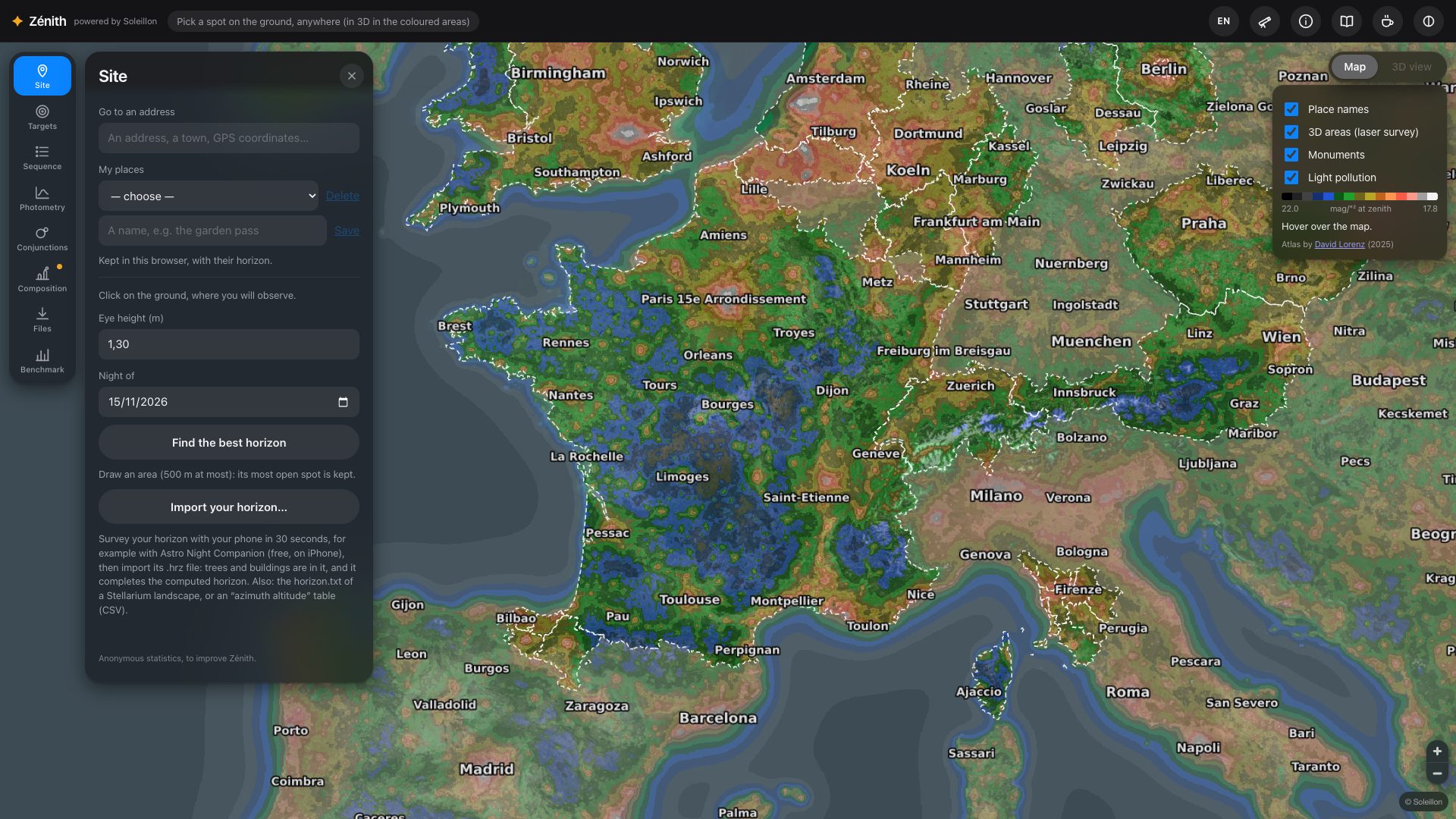
- Type an address, a town or GPS coordinates in Go to an address (Site panel), or zoom in on the map.
- Click on the ground where you will stand. Zénith reads the laser survey around that point, then the relief up to tens of kilometres, and computes your horizon degree by degree (a few seconds locally; the first time a site is read, up to about half a minute).
- Check your eye height (1.30 m by default) and the night you are planning.
- Give the spot a name and press Save in My places: it is kept in your browser with its horizon (and your terrain corrections, section 3), and coming back to it reloads nothing.
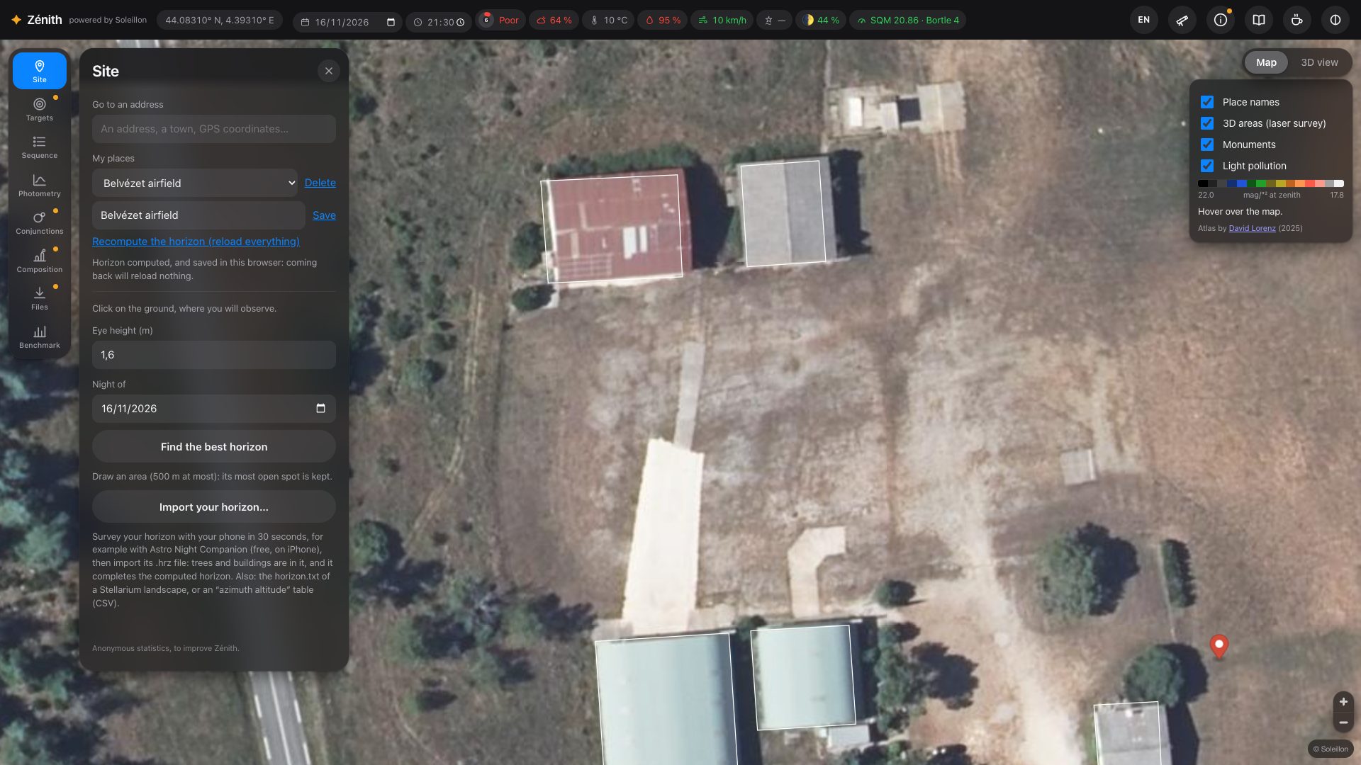
GPS coordinates and place names
Go to an address also reads coordinates, latitude first: decimal degrees (44.0831, 4.3931, or the French way
44,0831 4,3931; south and west negative) or degrees, minutes and seconds as Google Maps writes them
(44°04'59"N 4°23'35"E). With the letters N, S, E, W, the numbers can come in any order. One line is offered
(“… — GPS coordinates”): click it and the map goes there, as for an address.
When you zoom in, the map names towns, villages, hamlets and localities all over the world (OpenStreetMap), in the language of the page when OpenStreetMap has it, otherwise the local name. The Place names box of the map layers hides them.
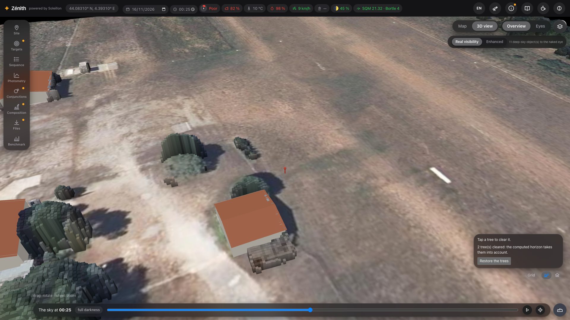
Zénith then switches to the 3D view. In Overview, you see the ground around you as the laser survey measured it, every tree and building at its real height, under the aerial photo. Drag to rotate, use the wheel to zoom.
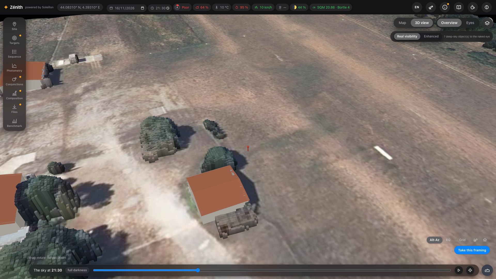
Where the laser surveys are read: France (IGN LiDAR HD), the Netherlands, Flanders, North Rhine-Westphalia, Hesse, Saxony-Anhalt, Rhineland-Palatinate, Brandenburg and Berlin, Switzerland, Austria, Czechia, Luxembourg, England, Wales, Scotland (partial coverage), Norway, Estonia, Tuscany, Navarre, the Basque Country, the United States (USGS 3DEP) and Canada. The dashed line on the map shows them.
Outside the LiDAR areas, you can still set a spot anywhere in the world: Zénith then computes the horizon from the relief only (and OpenStreetMap buildings of known height), and says so everywhere (“degraded mode”).
2. The top bar: your night at a glance
Once a spot is set, the top bar sums up the sky you are looking at. Hover any value for its details.

| Value | What it tells you |
|---|---|
| Coordinates | Your spot. |
| Date and time | The night and the time of the sky shown. Both are editable: type a date to change night, a time to move the sky. |
| Score ring | The night's score out of 100 and its verdict (Astro Night Companion's model: clouds, seeing, Moon, humidity, sky background, wind). Hover it for the full list of findings. |
| Clouds, temperature, humidity, wind | The forecast for that hour (Open-Meteo, or MET Norway as a fallback). |
| Seeing | Computed from the forecast upper-air profile (turbulence, jet stream). A dash when the forecast has no upper-air data, with the reason on hover. |
| Moon | Its phase and illumination; hover for its age and altitude at that time. |
| SQM · Bortle | The zenith sky brightness at that time, Moon included (from your own SQM reading if you entered one, otherwise the atlas), and the Bortle class of the site without the Moon. |
Each value is coloured by its quality: green good, orange watch out, red poor. On the right: the language button, the equipment, the information panel, this guide, a Ko-fi link to support the project, and the red night mode.
Three languages
The page speaks English, French and German. The language button shows the current one (EN, FR or DE); click it for a menu where each language is written in its own name: English, Français, Deutsch. The change is immediate, without reloading, and your choice is kept in your browser. Until you choose, Zénith takes your browser's language if it speaks it (German for an Austrian or Swiss German browser, for example), and English otherwise. This guide exists in the same three languages: the book icon opens it in the language of the page, and the line under its title leads to the other two.
What's new
When Zénith has new or changed functions, a What's new in Zénith window lists them when the page opens, by theme; for the photometry, each calculation comes with its model and its sources in small print. Don't show again hides it until the next list; the cross, Escape or a click beside it only closes it for now. Your very first visit does not show it: you are discovering the whole site, not what changed.
3. The 3D view at eye level, and the night
Press Eyes to stand at your spot. Drag to look around, use the wheel to narrow the field. The sky is drawn at the time shown in the time slider at the bottom: drag it through the night, press ▶ to play it, ⌖ to come back to the target. The label next to the time says where you are in the night (twilight, full darkness…).
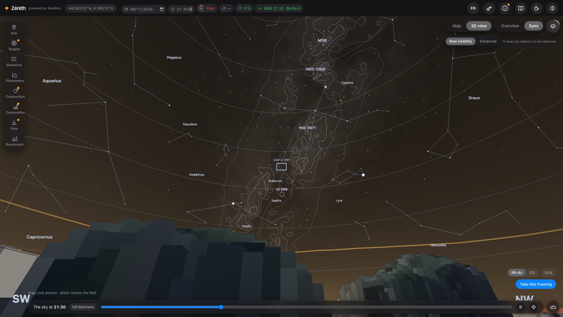
The wheel narrows the field down to 1°: enough to see the shape of a galaxy or a nebula.
Real visibility or Enhanced
Two buttons at the top right choose what the sky is for:
- Real visibility: what your eye can hope to see from here, tonight. The sky and the Milky Way are photometric, with no setting, and only the deep-sky objects that pass the eye's threshold are drawn (section 5).
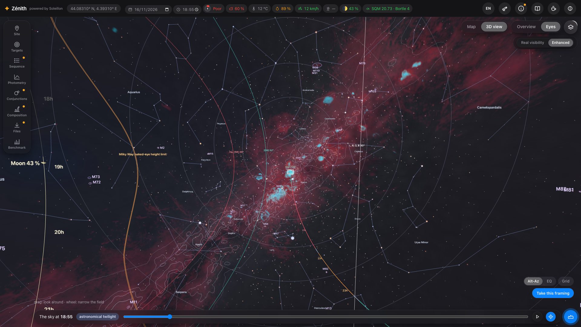
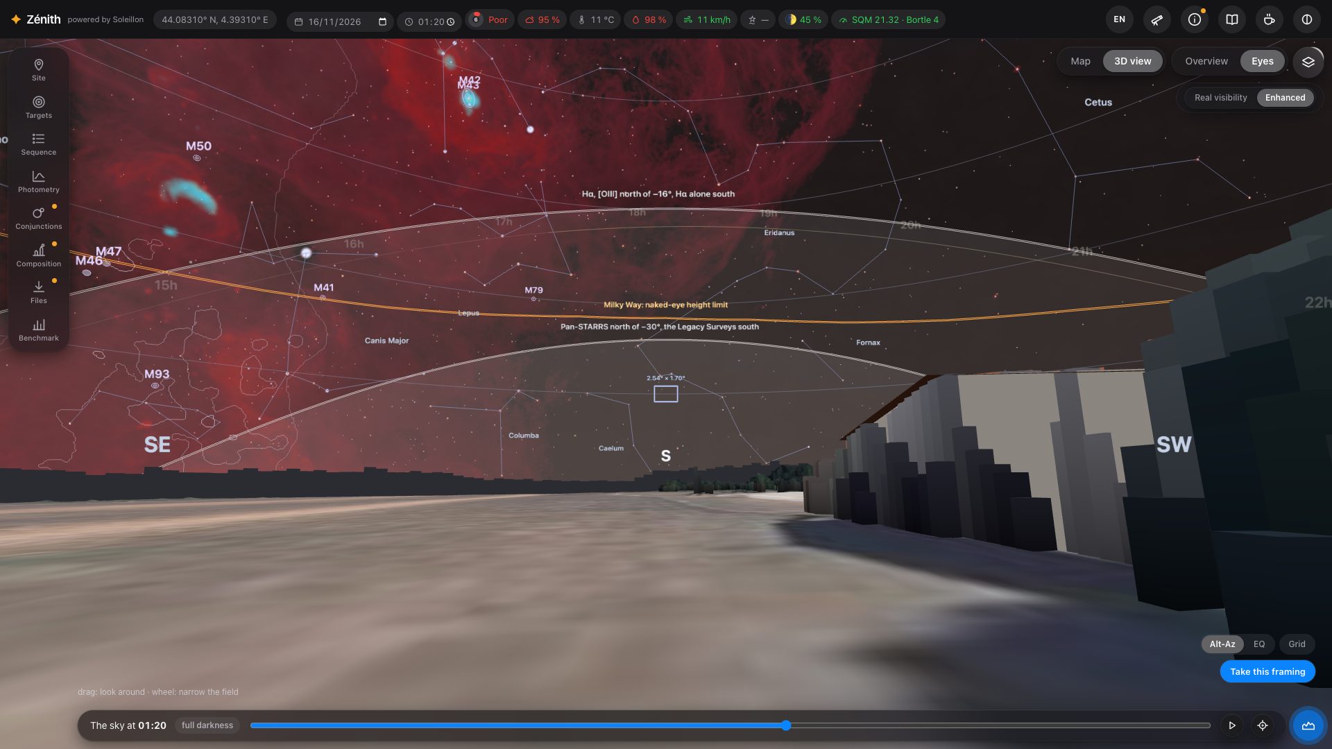
- Enhanced: the richest view, with nothing of the eye. The catalogues you tick, all the stars, the Milky Way and the objects at their measured light, the sky background removed (like an exposure with its background subtracted). The Hα and [OIII] clouds are drawn there, in a “ForaxX” HOO palette: red hydrogen, blue-green oxygen (section 4). Stars grow a little as you zoom in.
The real shape of deep-sky objects
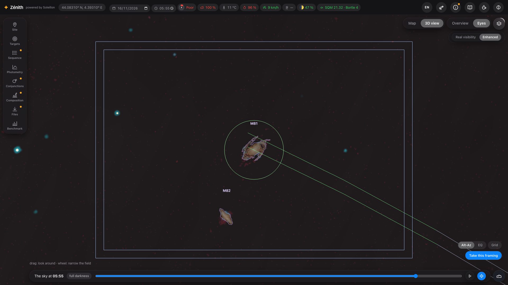
Zoom in on a galaxy or a nebula: instead of the catalogue's ellipse, Zénith draws its real outline, traced on Pan-STARRS images, filled with its measured light. Objects larger than one Pan-STARRS cut-out are assembled as a mosaic. Open clusters show their own stars, from Gaia DR3.
The mount and the coordinate grid
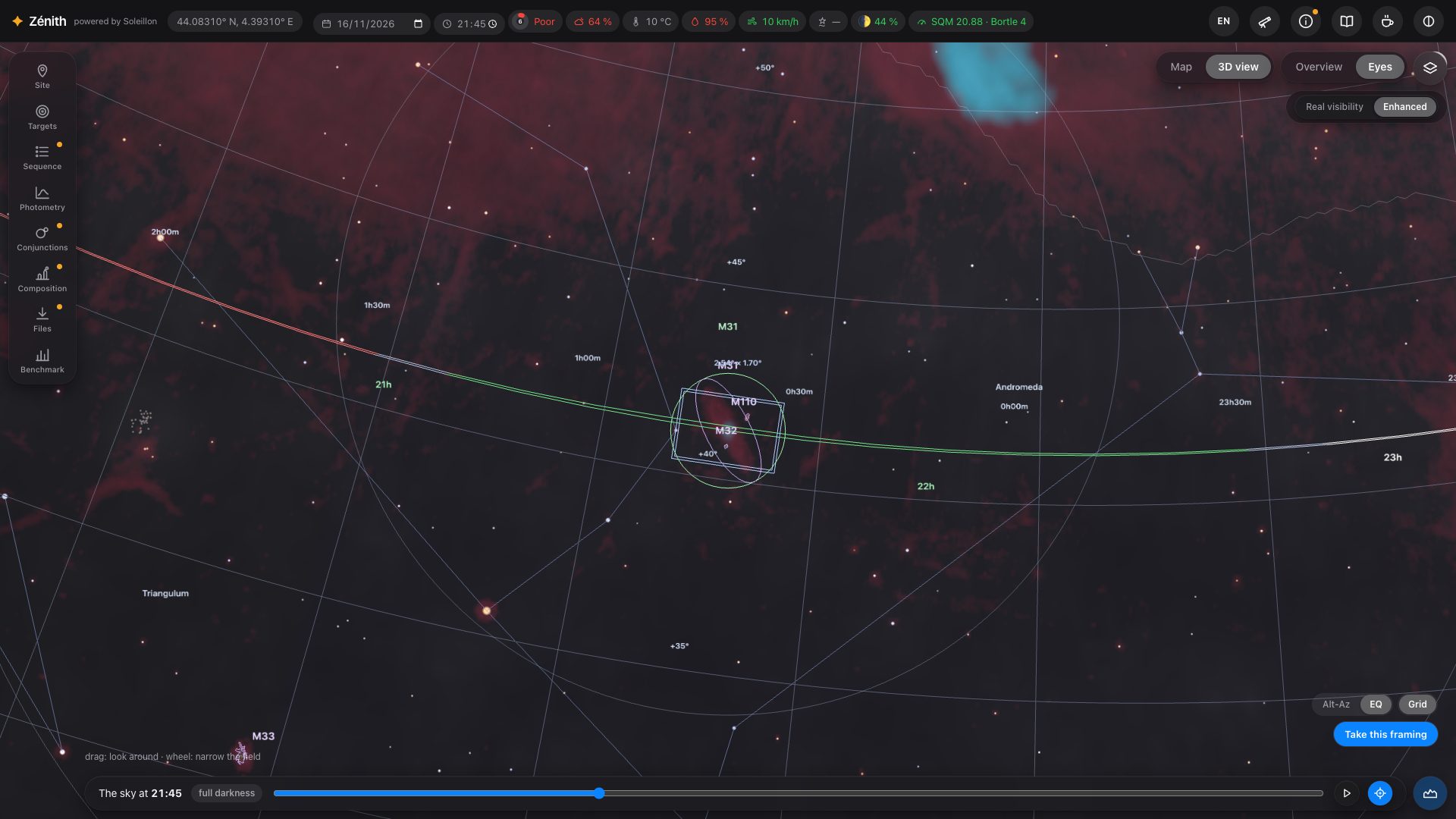
At the bottom right, Alt-Az / EQ says how your mount carries the camera: an alt-azimuth mount keeps the frame's top towards the zenith (it turns on the sky during the night), an equatorial mount keeps it towards the celestial north. Grid draws the matching coordinate grid: altitude and azimuth, or J2000 right ascension and declination. Its spacing follows the zoom, from 15° down to a few arcminutes.
The horizon profile
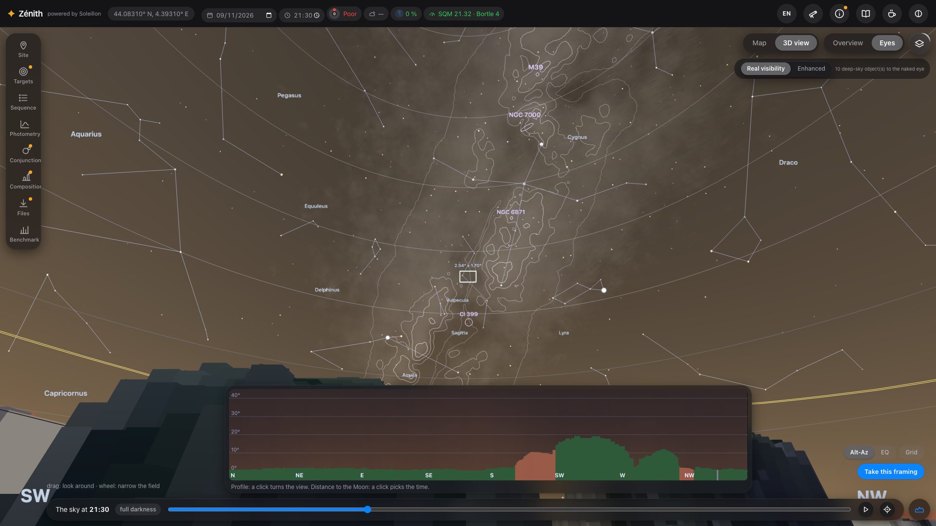
The button at the bottom right opens the profile of your horizon: its height all around, in the colour of what blocks the sky (grey terrain, green vegetation, red buildings). Click the profile to turn the view towards that direction.
Correcting the terrain: trees cut down, a new building
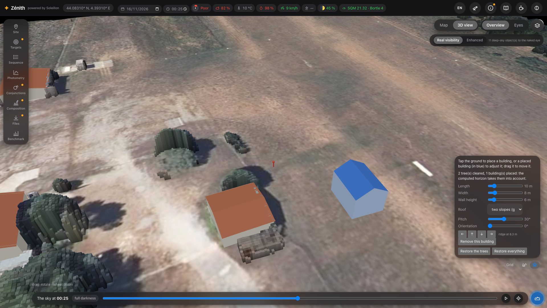
A laser survey is a few years old: a tree may have been felled since, a shed built. In Overview, on a spot inside a LiDAR area, two small tools sit next to the mount and the grid:
- Clear trees (the digger): touch a tree and it is cut down whole, with the vegetation joined to it (a hedge, over 6 m at most). Restore the trees puts them all back.
- Add a building (the house): touch the ground to set a building the survey does not know; it appears in blue. Set its Length, Width, Wall height and Roof: flat, single slope, two slopes (gable) or four slopes (hip), with the Pitch of its slopes (5° to 60°). Its ridge height is given under the arrows.
- To place it exactly, drag the building in the view (the view does not turn while you do), or nudge it 50 cm north, south, east or west with the arrows. Orientation turns it all the way round, 0° to 359° (a single slope has a direction). Touch a blue building to set it again; Remove this building takes it away, Restore everything undoes every correction.
After each change the horizon, its profile and the sky are recomputed, and everything that depends on them follows (the hours a target is hidden, the sequence, the exposure times). The corrections go with the spot, and with the place when you save it in My places. A building on top of you is refused.
4. Layers
The layers button (top right of the 3D view) chooses what is drawn on the sky.
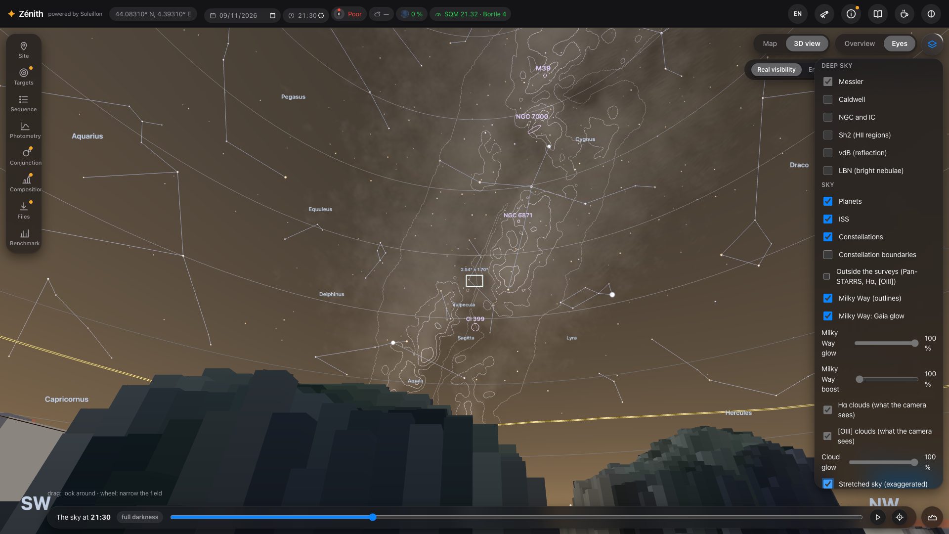
- Deep sky: the catalogues drawn in Enhanced (Messier, Caldwell, NGC/IC, Sh2, vdB, LBN). In Real visibility, only the objects you can hope to see with the naked eye.
- Sky: planets, constellation lines and boundaries, the Milky Way (outlines and Gaia glow), its naked-eye height limit, the target's path, the Moon's path and its avoidance zones, satellites (Starlink and OneWeb, off by default), light domes and their brightness contours, the Moon's light on the sky (Moonlight).
- Hα clouds and [OIII] clouds: ionised hydrogen and oxygen, north of −16° from the Northern Sky Narrowband Survey (Ziegenbalg 2025), south of it Finkbeiner's Hα map. Drawn in Enhanced only: the eye is almost blind to them at night. Finer when you narrow the field (“Detailed clouds…” while it loads). Cloud glow sets their strength.
- Milky Way boost: brightens the Milky Way where it dominates the sky, leaving its dark lanes as they are (a rendering choice).
- Outside the surveys (Pan-STARRS, Hα, [OIII]): greys the sky where the photometric analysis measures less well. South of −30°, the Legacy Surveys replace Pan-STARRS (in places) and SHASSA replaces the Northern Sky Narrowband Survey for Hα (dark veil); from −30° to −16°, Pan-STARRS and SHASSA (lighter veil). South of −16°, [OIII] is no longer measured. The northern limit of SHASSA (+15°) is drawn and named.
- Stretched sky (exaggerated): see section 5.
5. The photometric sky
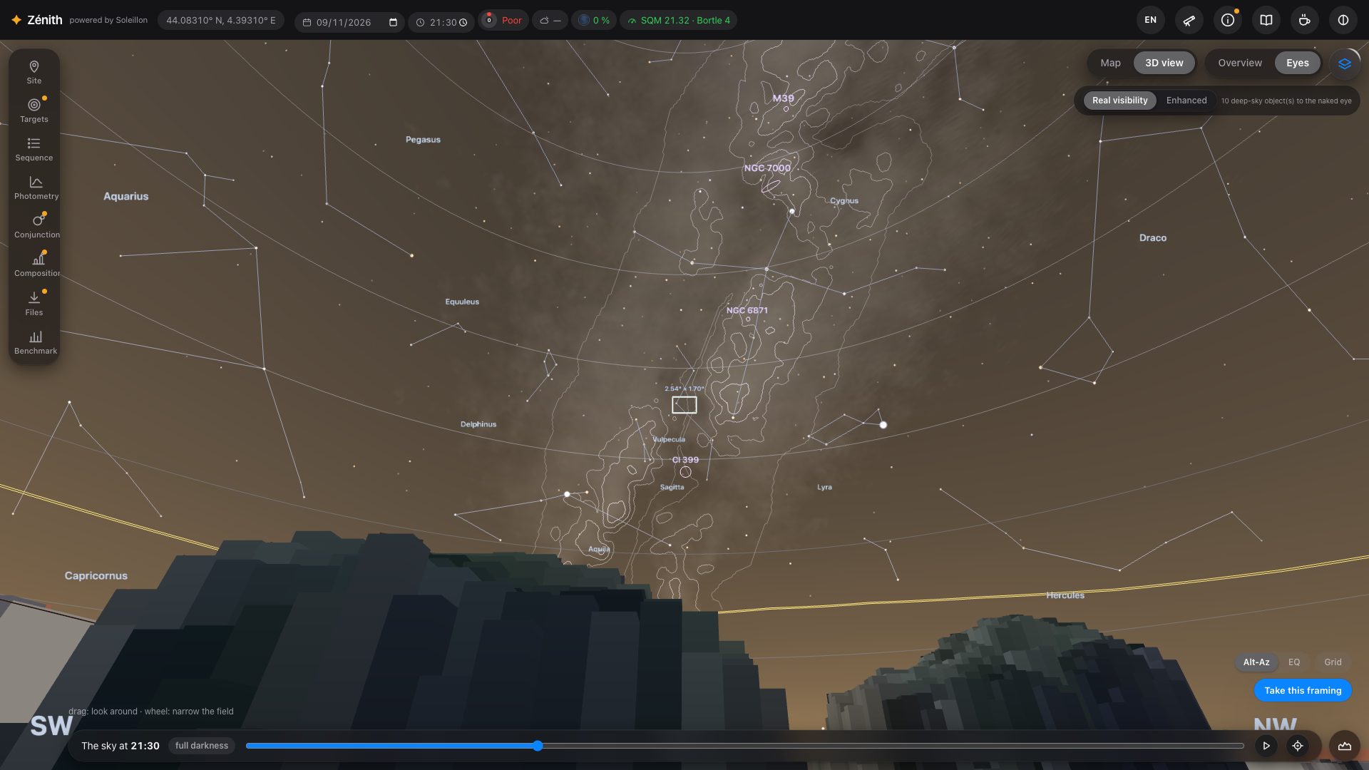
In Real visibility (top right of the view), the sky is not painted: it is computed in every direction from the natural sky (airglow scaled with the day's solar activity, zodiacal light, faint stars), twilight, the Moon, the light pollution and the air you look through. The same sky decides what your eye can see:
- each star is dimmed by the air it crosses and drawn only if it is brighter than the limiting magnitude of its own direction; a constellation line disappears with its stars;
- each deep-sky object is kept only if it passes the eye's contrast threshold (Crumey 2014) under the sky behind it;
- the Milky Way comes from the Gaia DR3 brightness map and is drawn against the local sky: it fades into light domes, moonlight and the thick air near the horizon. The orange line is its naked-eye height limit: above it you can see the band, below it you lose it. Its outlines are only drawn where the eye can tell it from the sky, and not before the end of civil and nautical twilight.
From the sky to your screen
A dark sky is several hundred thousand times dimmer than a white screen. Zénith shows it with an adaptation model (Ferwerda et al. 1996): faithful, and very dark. Tick Stretched sky (exaggerated) in the layers to lift the dark tones gently, the same way everywhere: a polluted sky stays brighter than a dark one, and the Milky Way becomes easy to see. It is labelled as exaggerated because the eye does not see it that bright.
Light domes
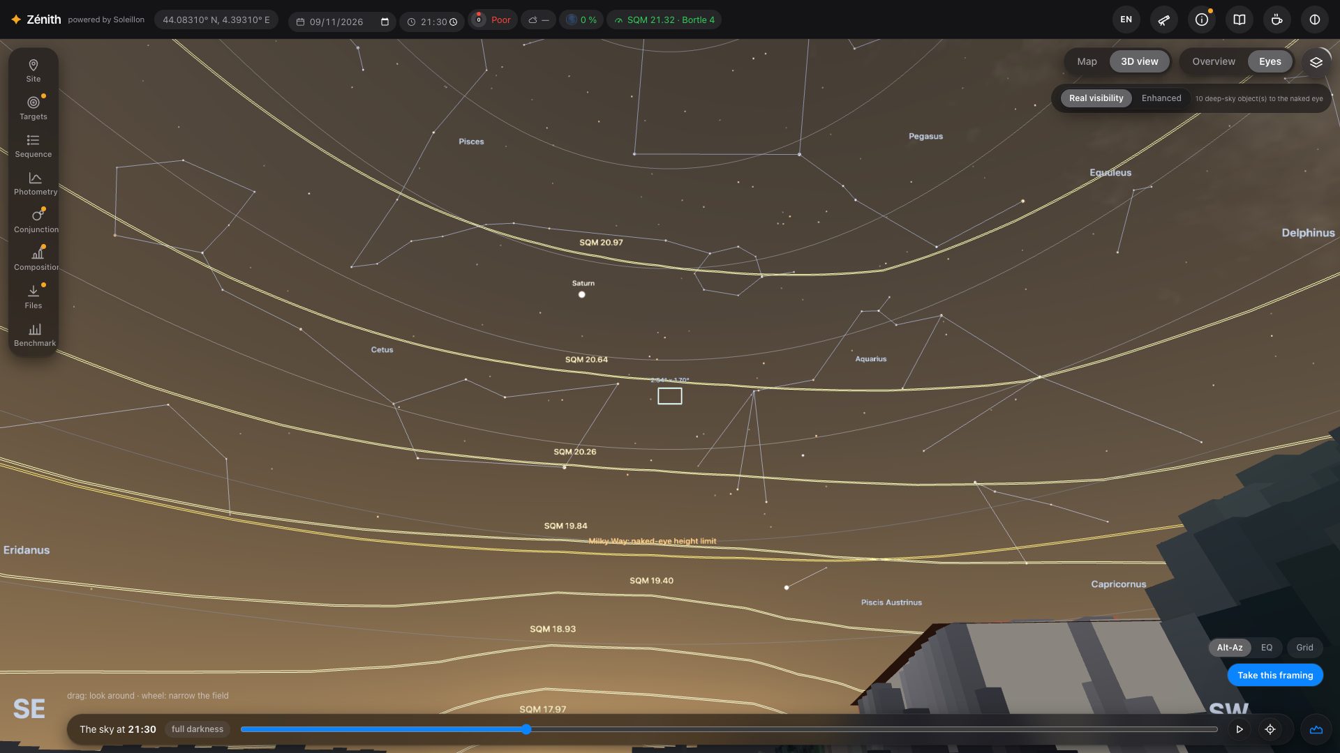
Towns appear as light domes in their real direction, from VIIRS satellite data. Tick Light domes: brightness contours to draw lines of equal brightness, each labelled with its SQM equivalent: you can read how high a dome climbs and how bright it is.
The Moon
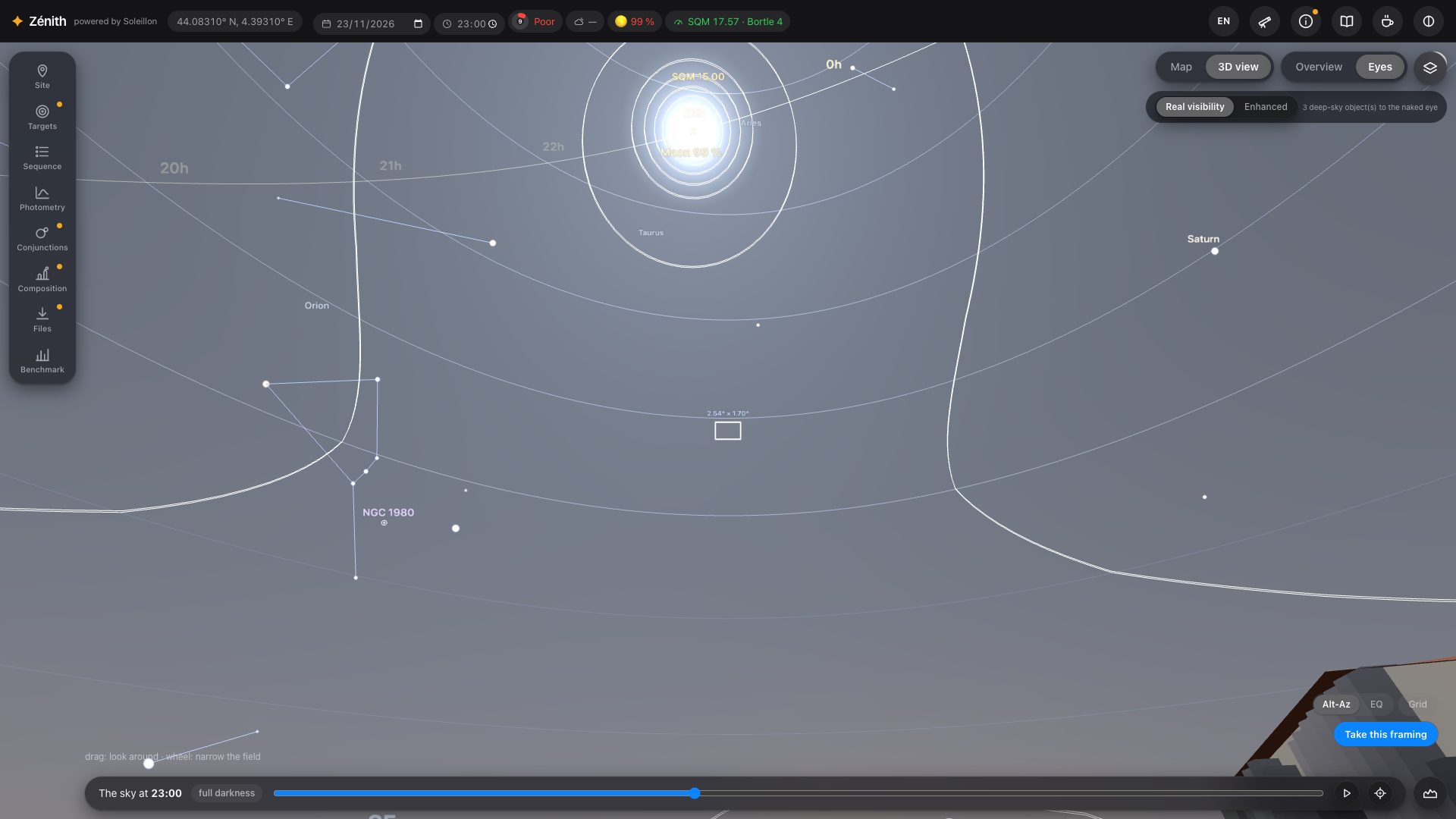
Moonlight is computed in every direction from its phase, its altitude and its distance to where you look (Krisciunas & Schaefer 1991). It brightens the whole sky, hides faint stars and objects, and counts in every SQM value. The circles around it are the Moon avoidance zones of your filters, each computed for its own filter (section 10).
Weather forecast (top right of the view): tick it to put the forecast aerosols (CAMS) in the extinction. The forecast is given for a cell about 45 km wide above its average relief; Zénith brings it down (or up) to the altitude of your spot, as aerosols thin out with height much faster than the air itself (a scale height of about 1.4 km). Without the forecast, a clear atmosphere is assumed, also thinner on a summit. A forecast, not a measurement. The cloud cover is shown as information only: it enters no computation.
6. Information
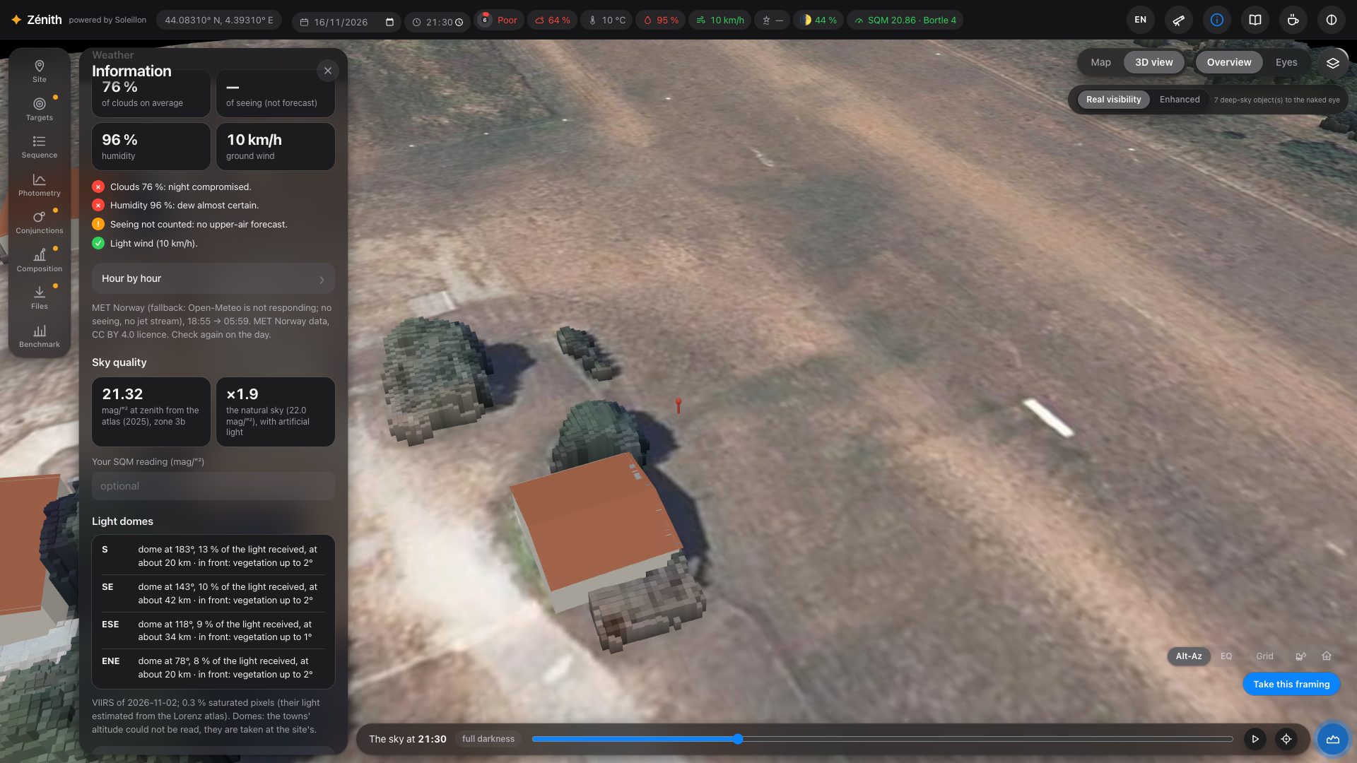
The i button in the top bar opens what Zénith knows about your spot.
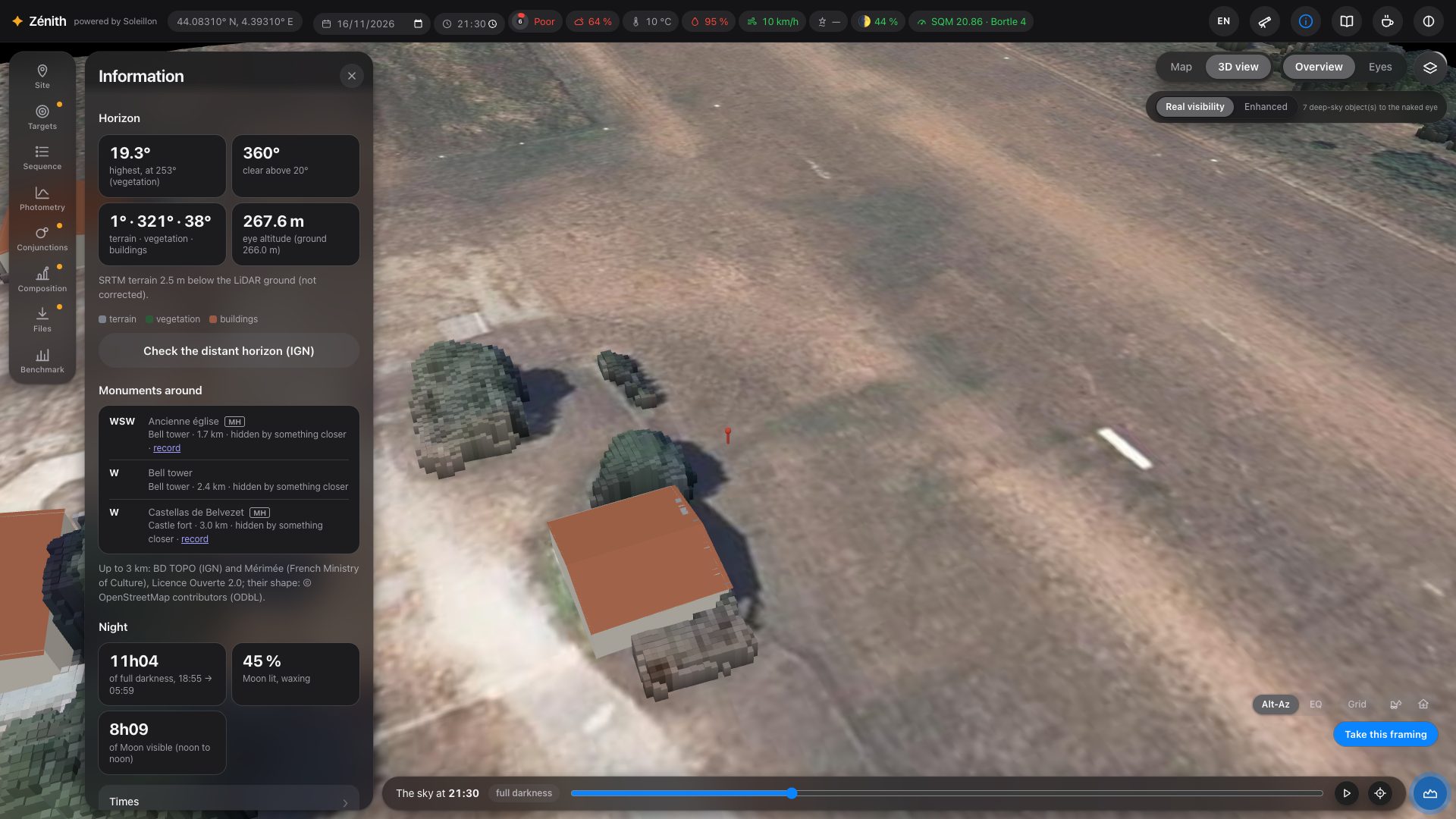
- Horizon: the highest obstacle, the share of directions clear above 20°, terrain / vegetation / buildings, your eye altitude, and a button that checks the distant horizon against IGN's finer elevation model (RGE ALTI, in France).
- Monuments around (up to 3 km), visible from here or not.
- Night: full darkness, the Moon, the times of the night.
- Weather: the night's findings and the hour-by-hour forecast.
- Sky quality: the zenith brightness from the atlas, and a field to enter your own SQM reading (it then replaces the atlas everywhere).
- Light domes: each dome's direction, share of the light, distance, and what stands in front of it.
7. Equipment
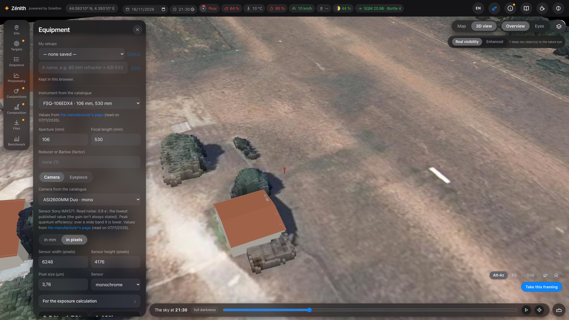
The telescope button in the top bar opens your equipment. Pick an instrument and a camera from the catalogue (values from the manufacturers' pages, with the link), or type them. Zénith computes the field, the sampling, the focal ratio and the resolving power, and draws your field frame in the 3D view. Save several setups under My setups.
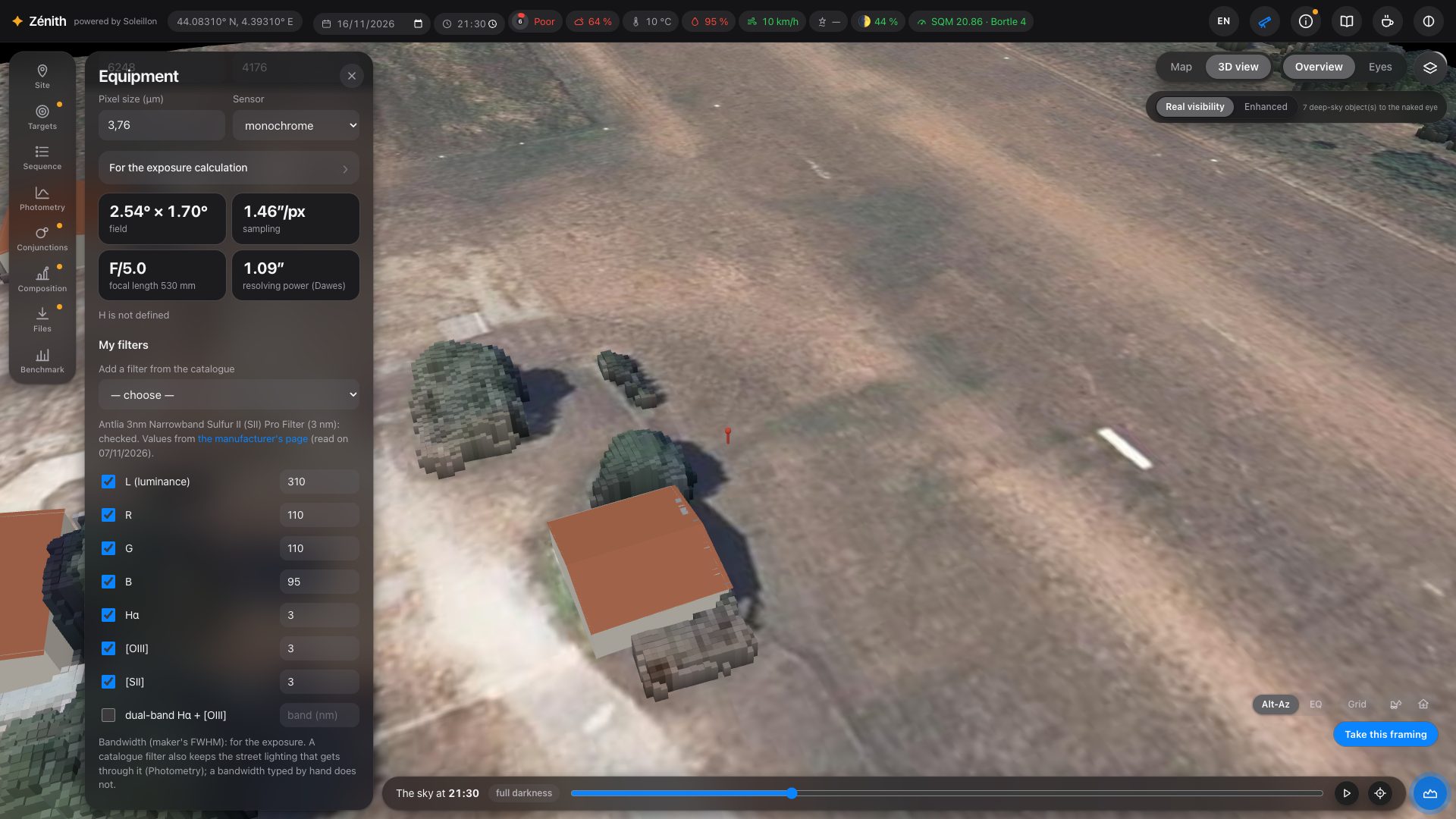
Then tick your filters (L, R, G, B, Hα, [OIII], [SII], dual-band Hα + [OIII]) with their bandwidth, or add them from the catalogue. A catalogue filter also knows how much street lighting, moonlight and natural night-sky light it lets through, which matters for the photometric analysis.
The sensor's response, and colour cameras
Under For the exposure calculation: the read noise, the quantum efficiency at its peak, the central obstruction, and the Sensor response curve. A catalogue camera takes the curve of its sensor by itself, from the SPCC database of Siril (the manufacturers' published curves). With it, each filter gets the efficiency of the sensor at its own wavelength: a monochrome IMX571 gives much less at Hα and [SII] than at its peak, and the times say so.
A colour (Bayer) camera is computed colour by colour: each line falls on its own pixels of the matrix (Hα on the red, one pixel in four; [OIII] on the green, two in four, and the blue), at that colour's response, leaks included. This works without a filter, with a dual-band filter, or with a single narrowband filter in front of the colour sensor. Without a narrowband filter, an emission nebula is still planned, in broadband with its sky background, and the note says so.
8. Targets
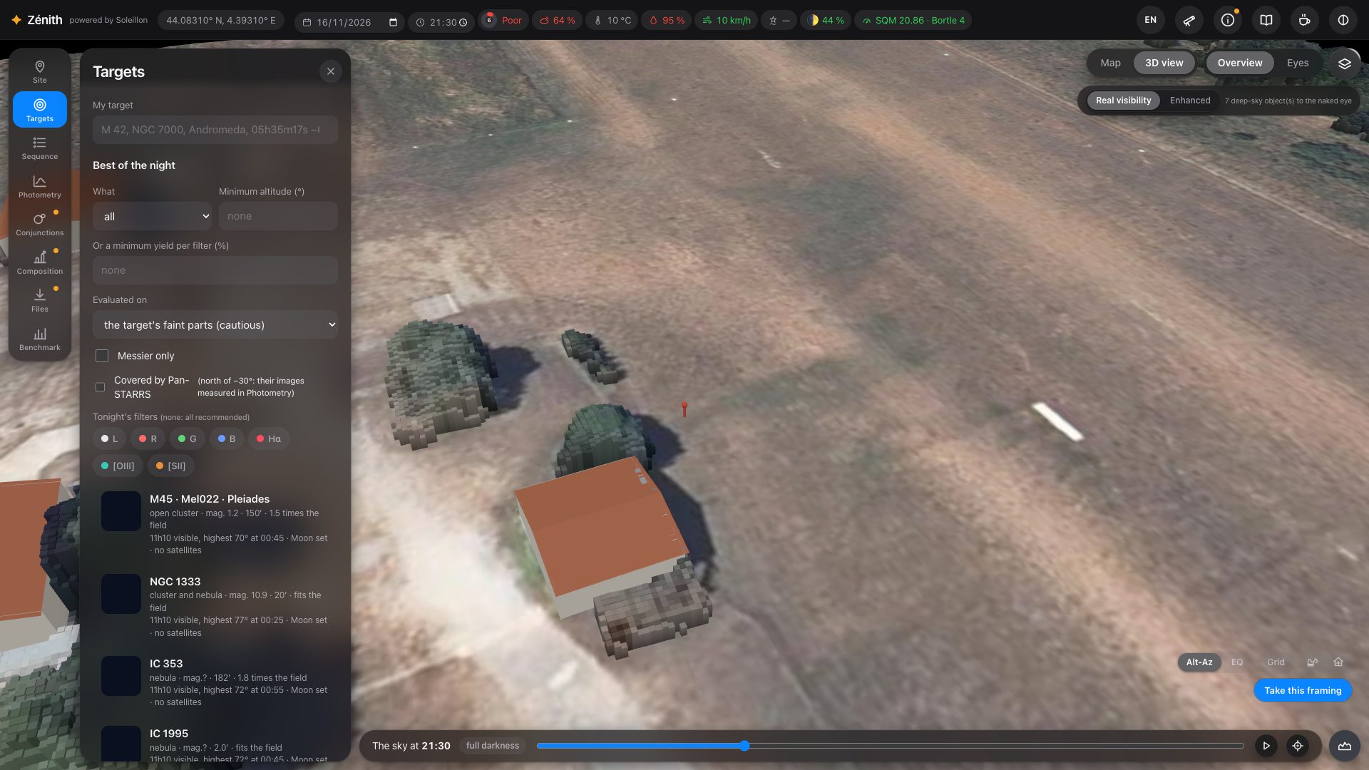
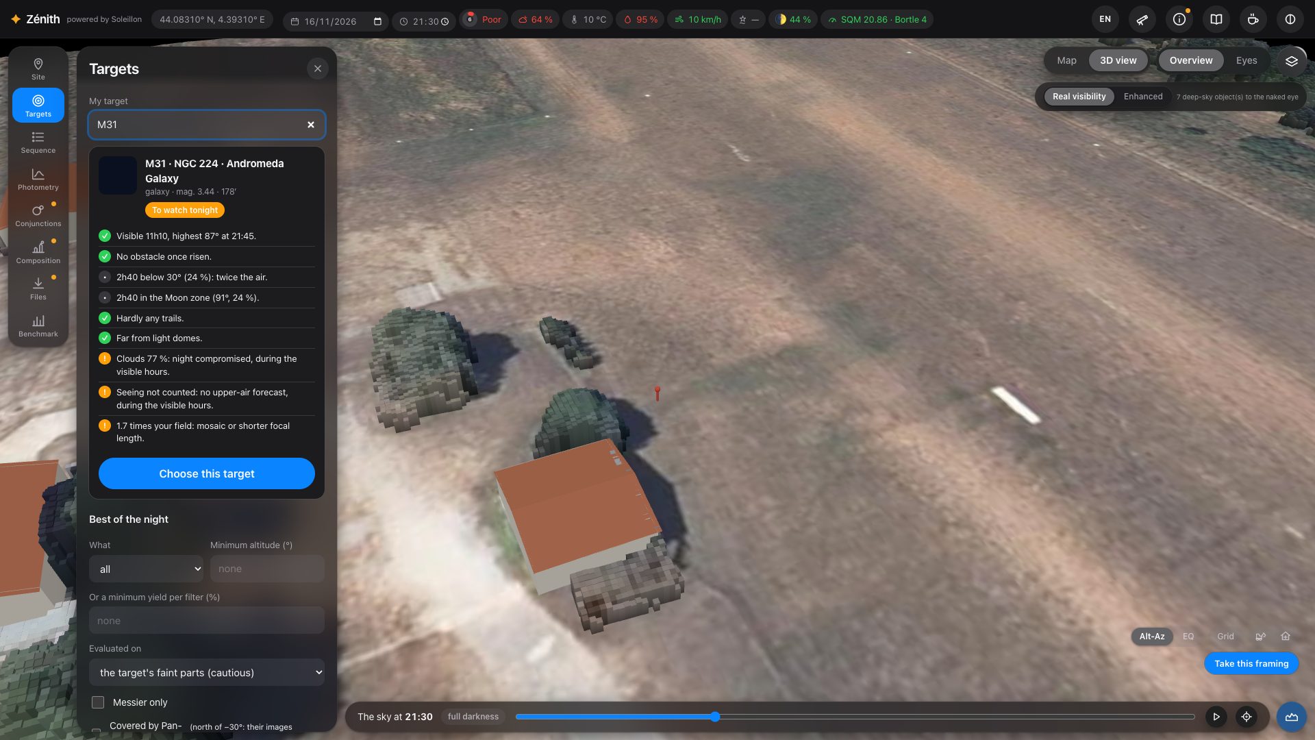
Targets lists the best objects of the night from your spot: how long they are visible above your real horizon, their highest altitude, the Moon, and the share of the time crossed by satellites. Filter by type, minimum altitude, minimum yield per filter, Messier only, or objects covered by Pan-STARRS images (for the photometric analysis).
My target
Type a name in My target (“M 31”, “NGC 7000”, “Andromeda”…) for its verdict tonight: visibility, obstacles, time low in the sky, Moon zone, satellite trails, light domes, clouds and seeing. Its path through the night is drawn on the sky, hour by hour. Press Choose this target to build its sequence.
9. Framing and the target's window
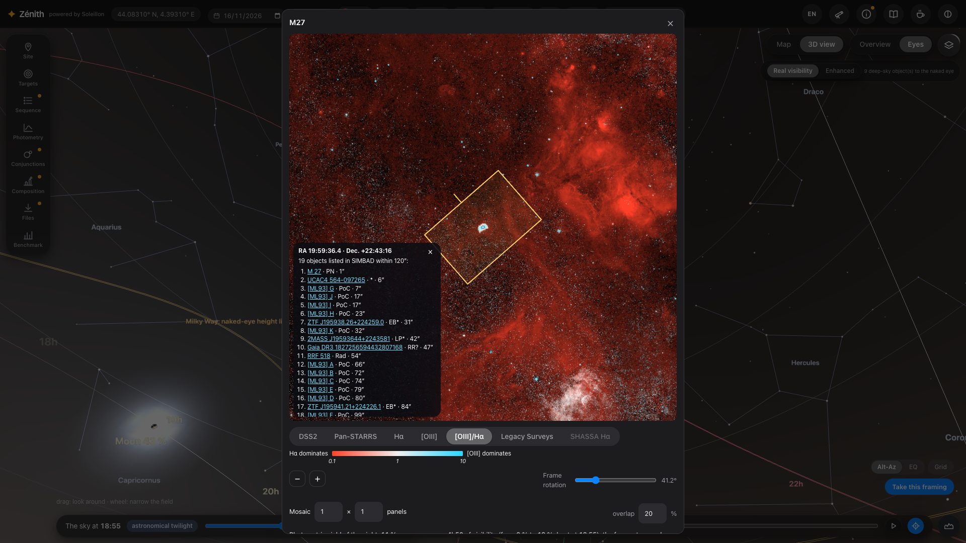
With a camera in your equipment, the blue frame of your sensor is drawn at the centre of the view. Drag the sky to move it anywhere, with or without a chosen target, then press Take this framing (bottom right). A window opens on that spot of the sky, the frame laid on an image of it.
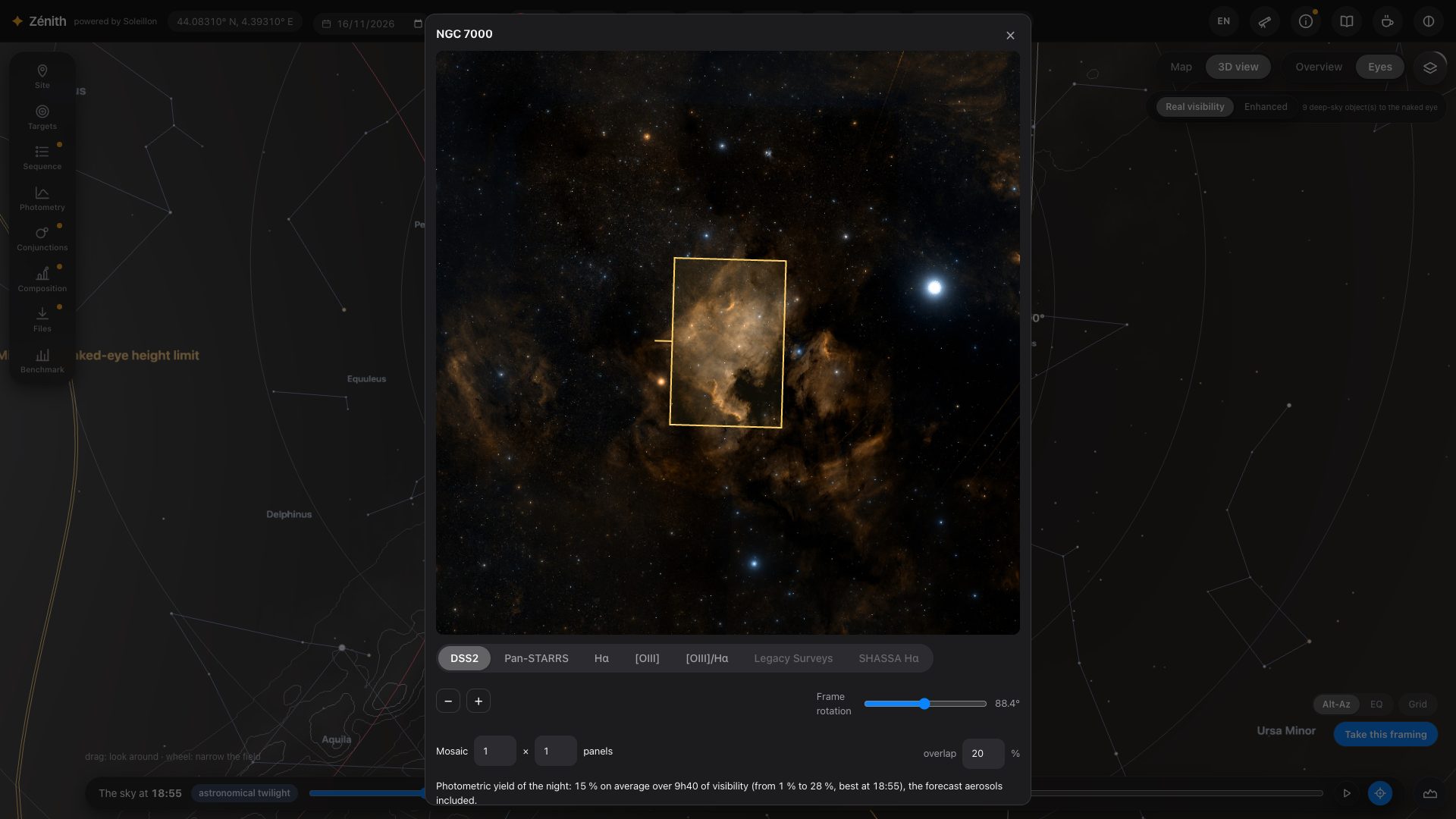
- The surveys: DSS2 in colour; Pan-STARRS (north of −30°); Hα and [OIII] from the Northern Sky Narrowband Survey (north of −16°); [OIII]/Hα, their ratio (below); Legacy Surveys (g, r, i like Pan-STARRS, deeper, south of +32°) and SHASSA Hα (the Southern H-Alpha Sky Survey Atlas, south of +15°). A survey with no data at these coordinates is dimmed but still clickable: chosen, its caption says so and DSS2 is shown instead.
- The frame: drag it on the image, turn it, make it a mosaic with its overlap. The centre and the angle are given in J2000.
- Send to the sequence keeps the framing (centre, angle, mosaic) for N.I.N.A. The view then draws the path of that framing through the night. A framing without a catalogued target becomes the “Frame target”, a target of its own at the exact centre of the frame.
- The filters chosen in the window are the ones the sequence takes.
The window shows the surveys and the framing only. How long to expose for a given extent and sharpness is answered in the Photometry panel (section 11), which takes up this framing: its sliders, its map of the target and its simulated image are there, and in the benchmark (section 15).
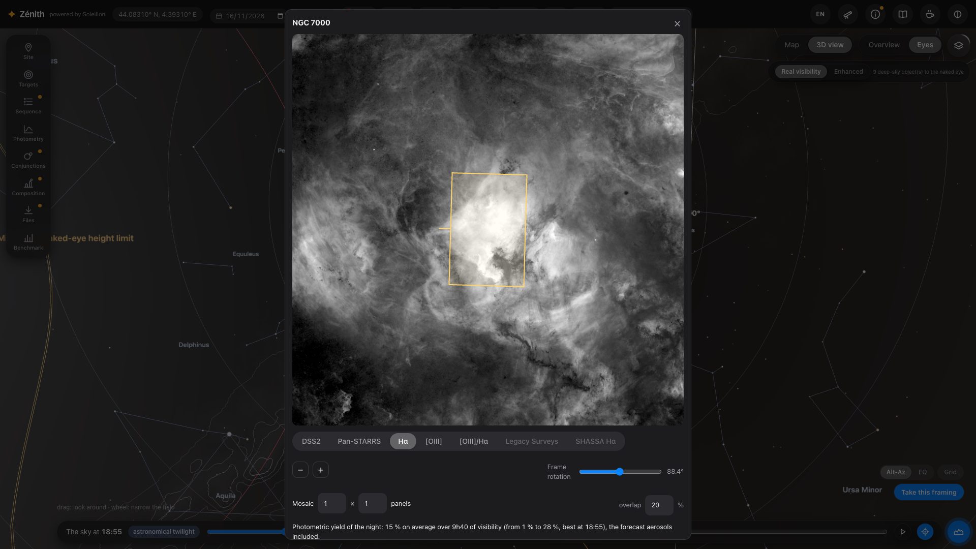
[OIII]/Hα: hunting planetary nebulae
[OIII]/Hα maps the ratio of the two lines, both already cleared of stars and continuum by the survey. The hue is the ratio: red where Hα dominates (an HII region), white when they are equal, cyan where [OIII] dominates, as in a planetary nebula. The brightness is the clearer of the two lines above the noise of the field: what stays in the noise stays dark. The ratio is in Rayleighs (photons); the survey's [OIII] calibration is approximate, and sources smaller than about 30″ are missing from it.
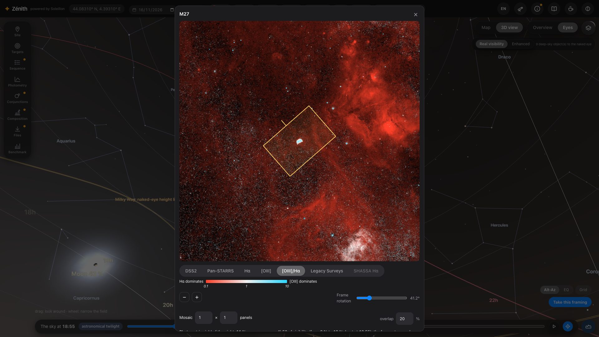
Right-click: is it in SIMBAD?
On any survey of the window, a right-click asks SIMBAD what is listed around that point, within a radius that follows the field (from 20″ to 2′), nearest first, with a link to each object's page. If nothing is listed, Zénith records a report for anteriority: the J2000 coordinates, the radius, the survey, the date and time, and the town of connection. The box says so.
10. Sequence, several nights, and N.I.N.A.
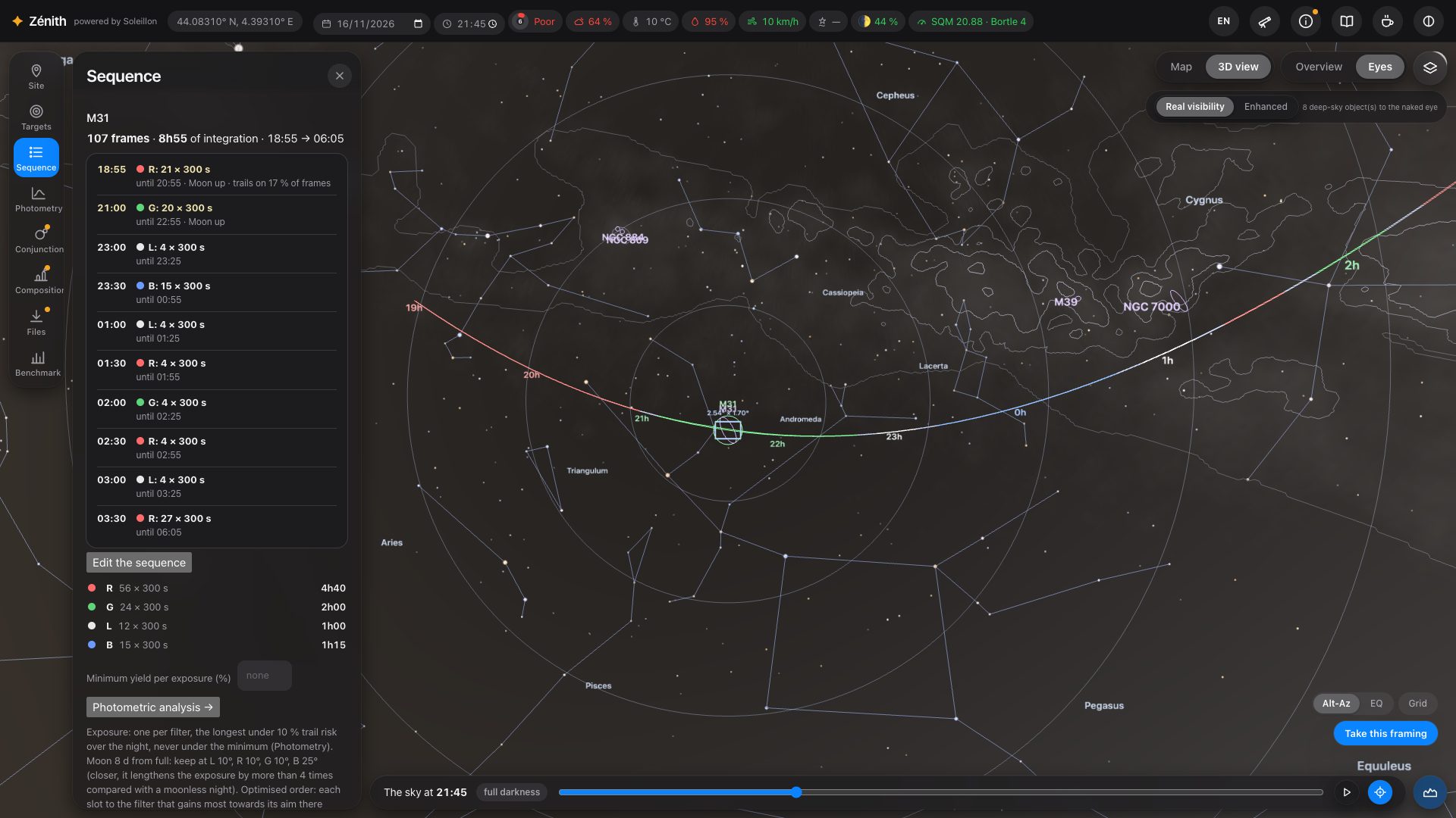
Sequence splits the night between your filters. Each filter has one exposure length for the whole night: the longest with
under 10 % risk of a satellite trail, never shorter than the minimum exposure that buries the read noise (Glover 2017). Edit it
freely, then export it to N.I.N.A. (Advanced Sequencer .json or Simple Sequencer .xml), with your
dithering, refocus and cooling settings.
Which filter, when
The night is not shared out evenly. Zénith cuts it into slots of 30 minutes and gives each slot to the filter that gains the most there towards its aim (the extent and sharpness set in Photometry, section 11): what that slot is worth to the filter, given the target's altitude, the extinction at its wavelength, the light domes in that direction and the Moon at its colour, compared with what it is worth to the others. The filter that is longest to fill gets more time; each gets its best slots. Neighbouring slots are joined into blocks, and each change of filter starts with 5 minutes of focusing. Typically Hα takes the hours with the Moon up, [OIII] the dark ones. The note under the sequence (“Optimised order…”) says so. Without a camera, a known sky background or a filter that can be computed, the sequence falls back to equal shares.
The Moon, filter by filter
The Moon avoidance zone is computed for each filter, at each moment the Moon is up: Zénith compares the sky background the Moon would add at every distance from the target with the same night without the Moon, in that filter (its colour depends on the distance). The zone is the distance within which the background is more than 4 times that of a moonless night. A narrow Hα filter can therefore work much closer to the Moon than [OIII] or broadband. If the Moon is too bright for every filter while the target is up, the sequence is empty and says why.
Minimum yield per exposure: set it (for example 50 %) and the times when the target gives less are left out; the sequence is redone on the rest. Edited by hand, the sequence keeps within the yield you asked for when you add filters.
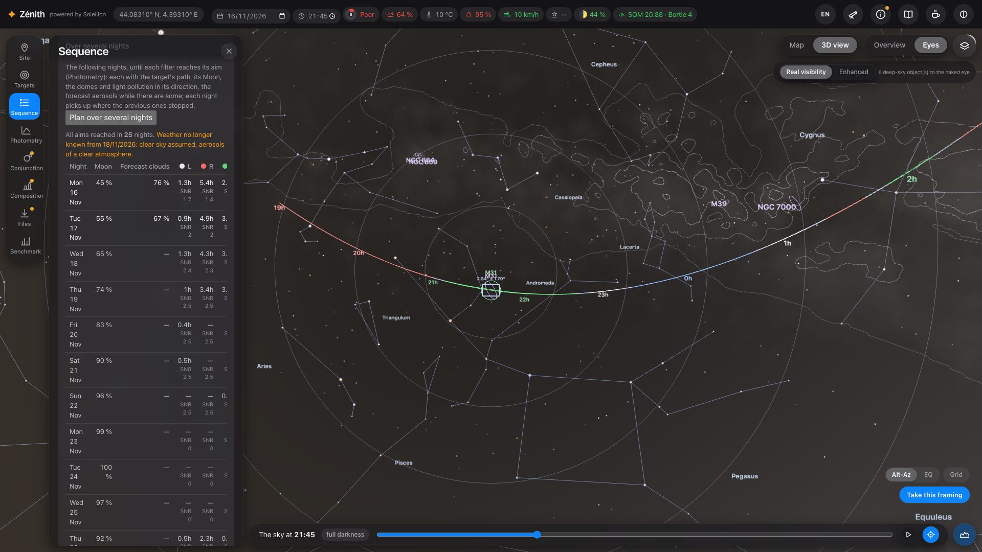
Over several nights
One night is rarely enough. Open Over several nights and press Plan over several nights: starting from the chosen date, Zénith plans night after night (30 at most), each with its own path of the target, its Moon and avoidance zones, the domes and light pollution of its direction and, while the forecast lasts, its forecast aerosols. Each night picks up where the previous ones stopped, until every filter reaches its aim.
One line per night: the date, the Moon, the forecast clouds, and for each filter the hours of exposure that night and the SNR reached since the first night. At the top: “All aims reached in N nights”, or the aims not all reached in 30 nights. Beyond the weather forecast, the lines are marked and the page says from when a clear sky is assumed. Clouds are shown to help you decide; they never enter the calculation.
11. Photometric analysis: how long to expose
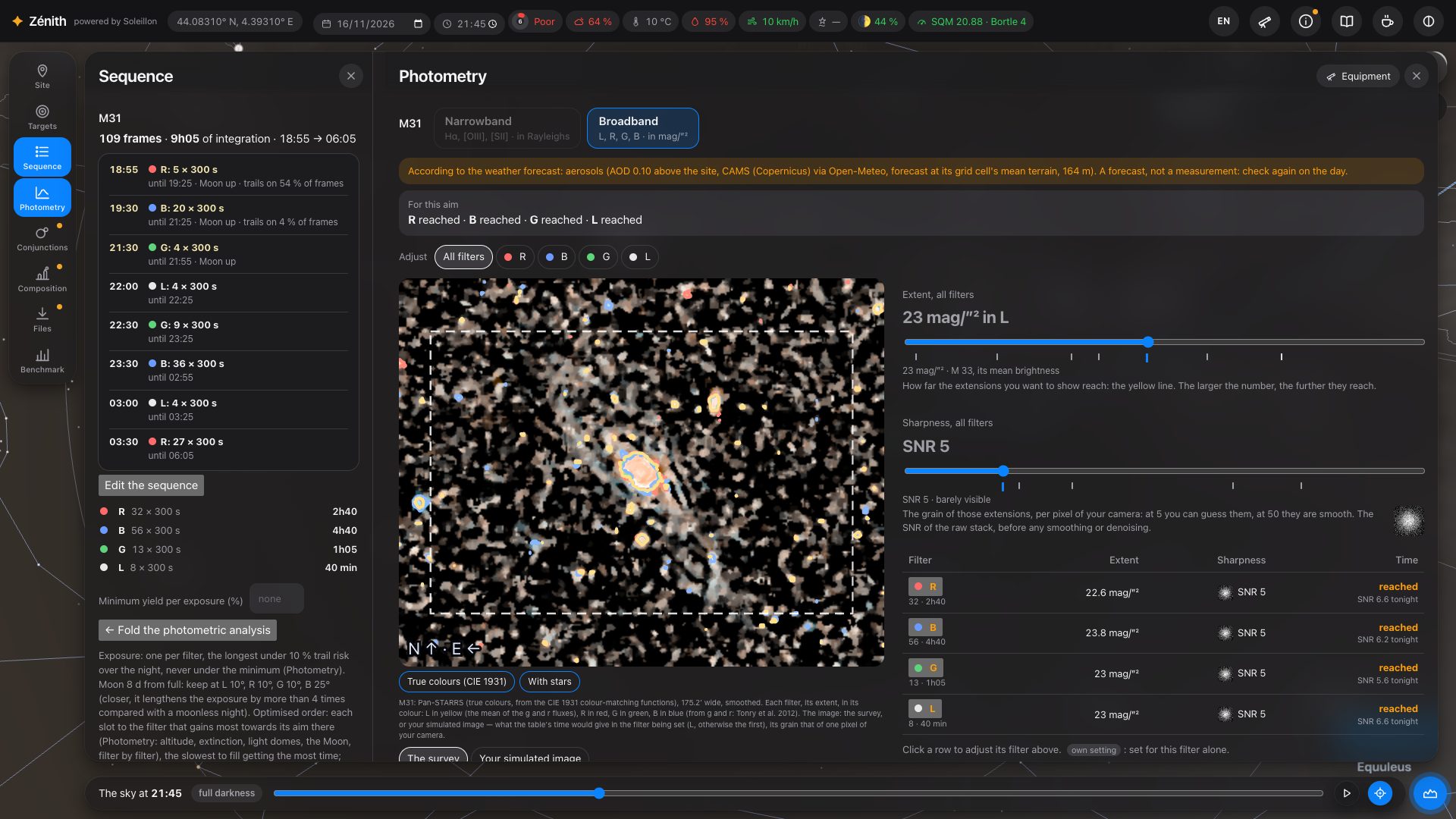
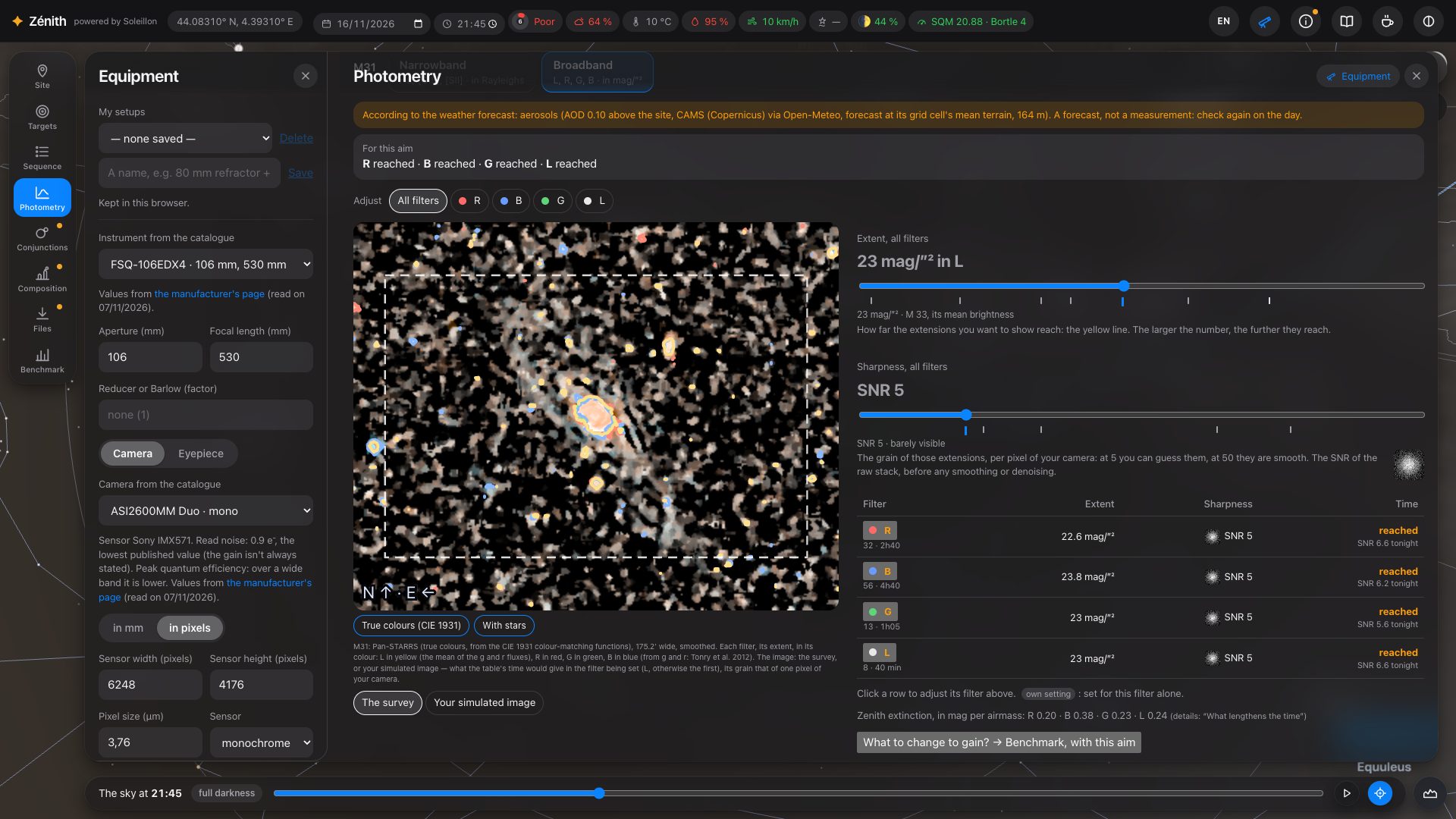
Open it with the Photometry icon (under Sequence), or Photometric analysis → in the sequence. It answers one question: from this spot, with this equipment and this sequence, how many hours do I need, in each filter, to show the target this far out, this cleanly? Two tabs: Narrowband (Hα, [OIII], [SII], in Rayleighs) and Broadband (L, R, G, B, in mag/arcsec²). Both work the same way.
Your aim: the extent and the sharpness
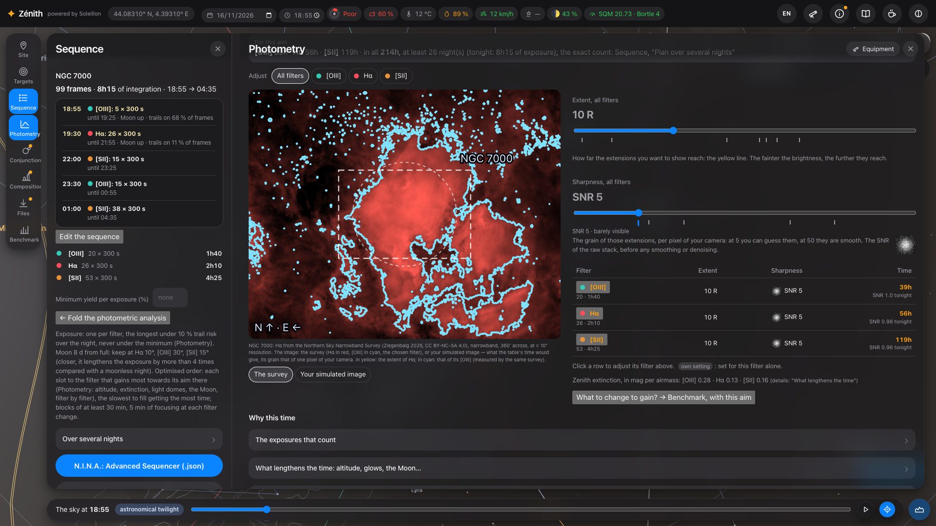
Extent: how far out you want to go: a surface brightness in mag/arcsec² for a galaxy, a line brightness in Rayleighs for a nebula. The matching isophote is drawn in yellow on the target's image; the dashed rectangle is your camera's field. Sharpness: the signal-to-noise ratio (SNR) of one pixel of your camera, all exposures stacked, before any smoothing or denoising (5: barely visible, 50: smooth). A square next to the slider shows the grain of a pixel at that SNR.
Under each slider, small marks help you choose: hover one for its name, click it to set the slider there. For the extent, the target's own bright parts (the brightest 5 % of its disc) and extended parts (the brightest quarter), read on its map; for the sharpness, the detection threshold and what award-winning AstroBin images reach (M 20, the Rosette, M 82), brought to your sampling. The examples of Orion (narrowband) and M 33 (broadband), folded, give reference brightnesses.
Adjust chooses what the sliders set: All filters, or one filter alone (“Extent in [OIII]”, “Sharpness in [OIII]”…): the other filters keep theirs. The aim is the same everywhere: the extent is kept per target, the sharpness for all targets, and the benchmark (section 15) reads and sets the same aim.
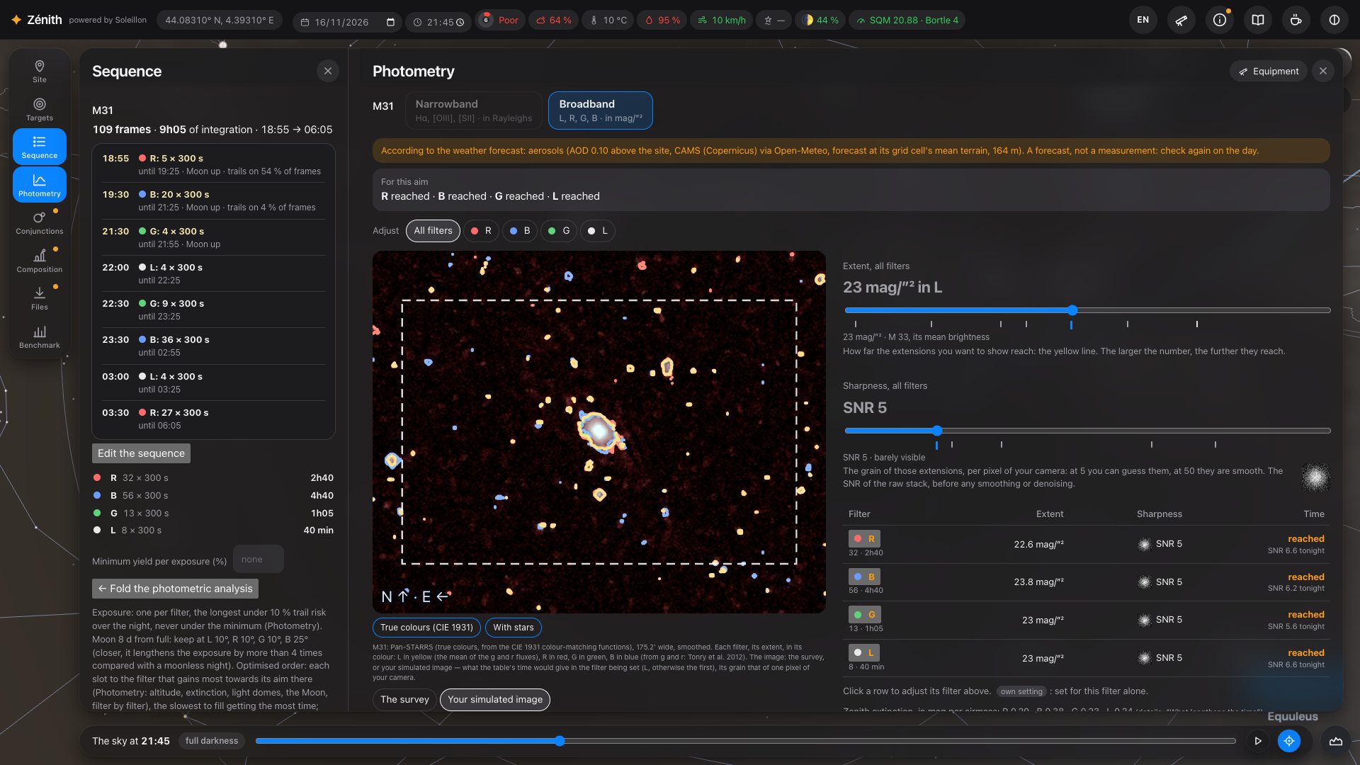
The image shows either The survey (the target's measured map, made readable) or Your simulated image: what the time of the table would give in the filter being set, with the grain of one pixel of your camera.
The time, filter by filter
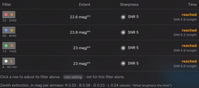
The table gives one line per filter: its extent, its sharpness (with its grain), and the exposure time it needs for that aim, with the SNR tonight's sequence gives. “own setting” marks what is set for that filter alone; click a line to adjust its filter above. Under the table, the extinction of each filter at the zenith. At the very top, the line For this aim repeats the time of each filter, then the total and the number of nights it takes at least, if every night exposed as much as tonight's sequence. The exact count, with each night's Moon and weather, is in Sequence, Plan over several nights (section 10).
Where the target's brightness comes from
Zénith measures the target on survey images, over the whole field of your frame:
- Broadband: Pan-STARRS north of −30°, the Legacy Surveys south of it, in true colours. Pan-STARRS cut-outs are assembled to cover your frame, up to 3°, and kept in your browser so the next visit is quicker; a target larger than that is measured in its centre, and the page says so. While they arrive, the DSS2 image and the catalogue's model stand in, with a notice.
- Hα: the Northern Sky Narrowband Survey north of −16°, SHASSA south of it, otherwise Pan-STARRS or the Legacy Surveys with the continuum removed, and as a last resort Finkbeiner's all-sky map (6′).
- [OIII]: the Northern Sky Narrowband Survey, or measured on Pan-STARRS; otherwise estimated from the shape of Hα and a ratio, drawn in cyan along the Hα isophote. [SII] and dual-band take the Hα map (no survey measures [SII]).
While maps load or the analysis computes, a line at the top says what is loading (“Loading: …”), how many tiles are in, and for how long; times and isophotes update when it arrives. When a filter cannot be computed, or a survey image cannot be read, the reason is written rather than an empty tab.
What the sky does in each filter
Every part of the sky background is passed through the band of each filter, not taken as flat:
- the natural sky has the spectrum of the night sky (ESO's SkyCalc model): a narrow [OIII] filter takes less of it than a flat spectrum would, Hα a little more (the OH lines);
- the Moon has the colour of its scattered light, which depends on its distance from the target: it weighs more in [OIII] and blue, less in Hα;
- the lamps of the towns around: choose sodium or LEDs in Lamps of the towns around; a light-pollution filter cuts sodium well, LEDs much less;
- the extinction is computed for each filter at its wavelength: the molecules of the air (much stronger in the blue), the aerosols at the altitude of your spot (forecast, or a clear atmosphere), and ozone. Extinction, filter by filter gives the three parts and the total.
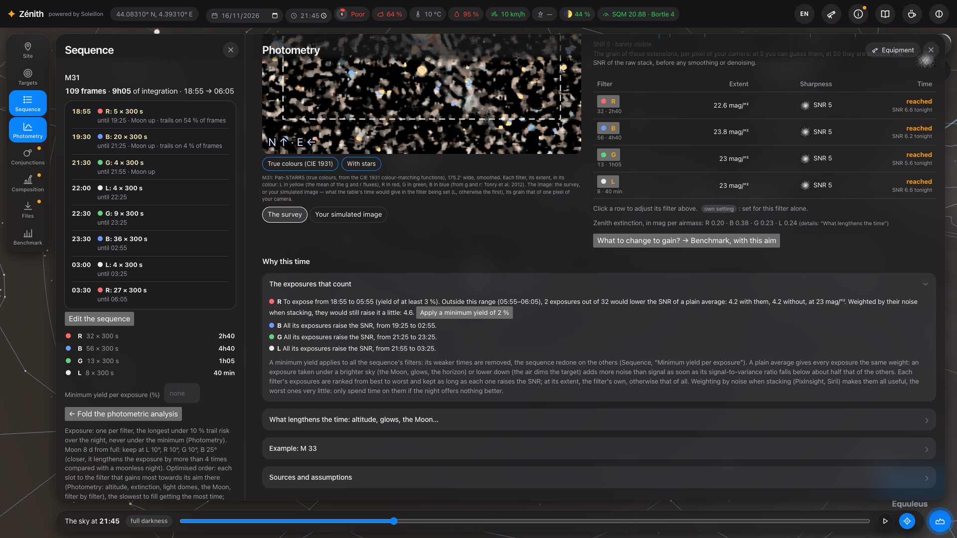
Why this time
Below the table, folded sections explain the result:
- The exposures that count: an exposure taken under a brighter sky or lower down adds more noise than signal once its quality falls below about half the others'. Each filter's exposures are ranked, and the analysis says which ones raise the SNR, and from when to when. With weighted stacking (PixInsight, Siril) the weaker ones still help a little.
- What lengthens the time: altitude, glows, the Moon…: the time here compared with the same SNR under an ideal sky (no light pollution or Moon, the target at the zenith), and what costs the most; Take the weather forecast into account (aerosols); the lamps; the yield through the night, filter by filter, hour by hour; and the extinction table.
- In narrowband, In broadband, for comparison (your broadband filters exposed like your Hα) and Advanced analysis: your target's [OIII]/Hα ratio, measured on Pan-STARRS.
Try other equipment, live
Press Equipment at the top of the analysis: your equipment opens in a narrow column on the left, and the analysis is recomputed at every change. Try another telescope or camera and watch the hours change. To compare two setups side by side, follow What to change to gain? → Benchmark, with this aim (section 15).
12. Conjunctions
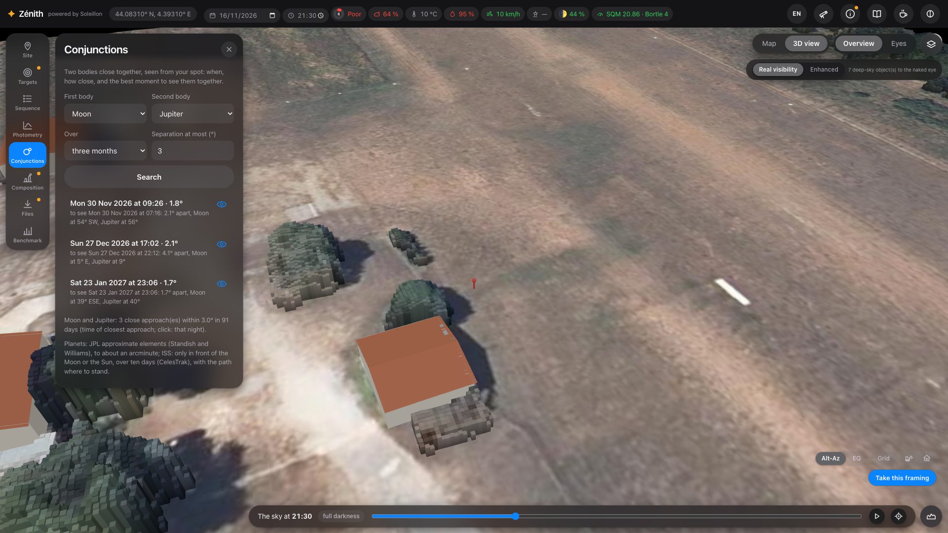
Two bodies close together, seen from your spot: the Moon, the Sun, the planets, bright stars and clusters (the Pleiades, Aldebaran, Regulus, Spica, Antares), and the ISS in front of the Moon or the Sun. Choose them, a period and a maximum separation, and press Search: Zénith gives the moment of closest approach and the best moment to see them together (both above your horizon, in the dark), with their altitudes.
13. Composition: a monument in the foreground
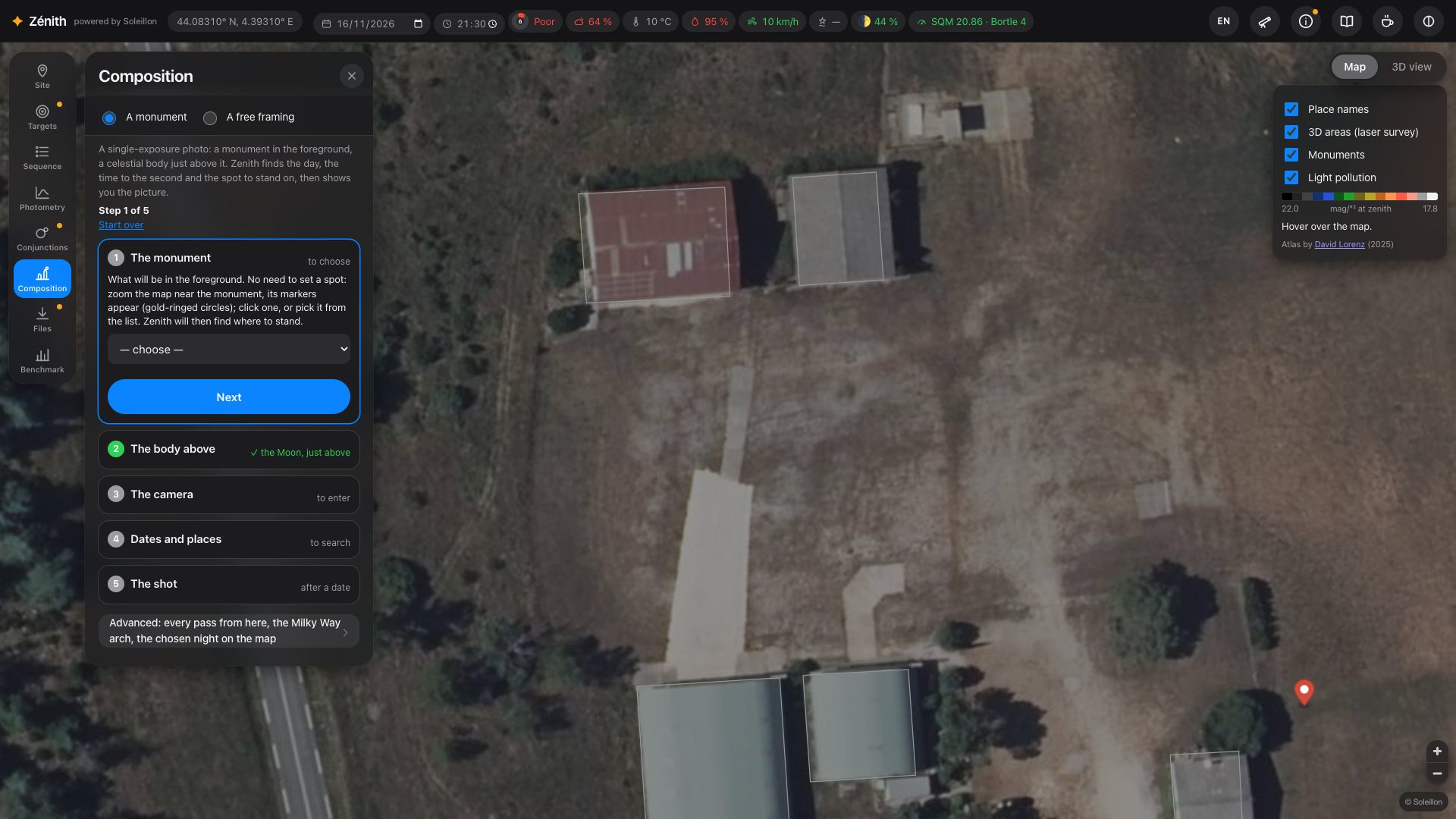
For a single-exposure photo with a monument in the foreground and a celestial body just above it. You do not need to set a spot first: Zénith finds the day, the time to the second, and where to stand.
- The monument: zoom the map near it and click its marker (gold-ringed circle), or pick it from the list (French national topographic database and historic monuments register; OpenStreetMap elsewhere).
- The body above: the Moon, the Sun, the Milky Way's core or arch, a constellation, a comet or a deep-sky object; just above the top, or with a gap.
- The camera: focal length, aperture and sensor.
- Dates and places: Zénith searches a whole year. The map shows in green where the top of the monument can be seen from, and dots where the body will sit on it.
- The shot: click a date. Zénith moves you to that spot, recomputes the horizon from there, checks that no tree or roof is in the way, and shows the frame at the exact second, with recommended settings.
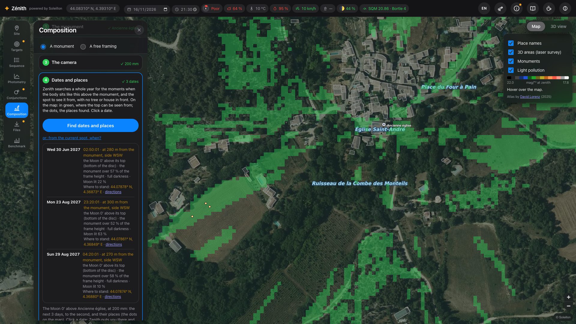
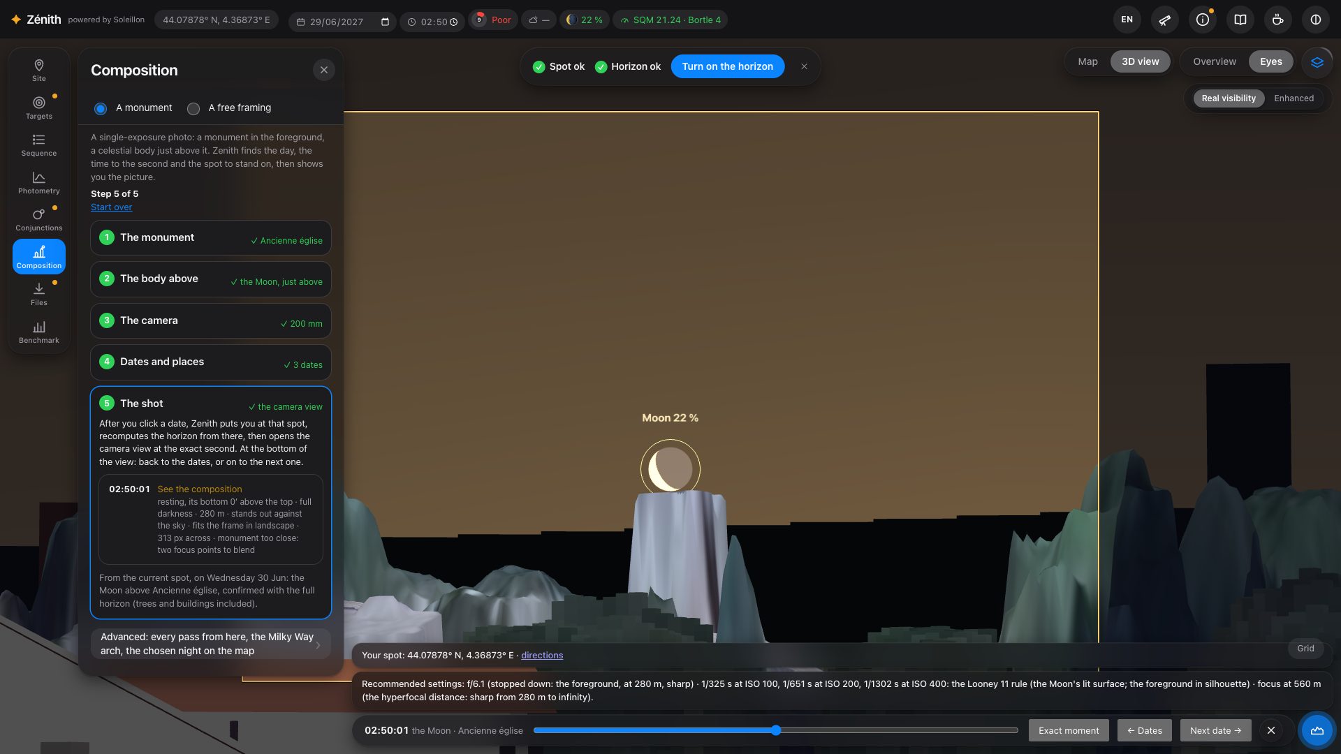
A free framing (second tab) does the same without a monument: a landscape, a street, a viewpoint; you frame it, Zénith finds when the body passes the chosen place in your frame. The Advanced section lists every pass from your current spot, the Milky Way arch rising behind a monument, and the chosen night on the map.
14. Files
Everything is made in your browser; nothing is sent.
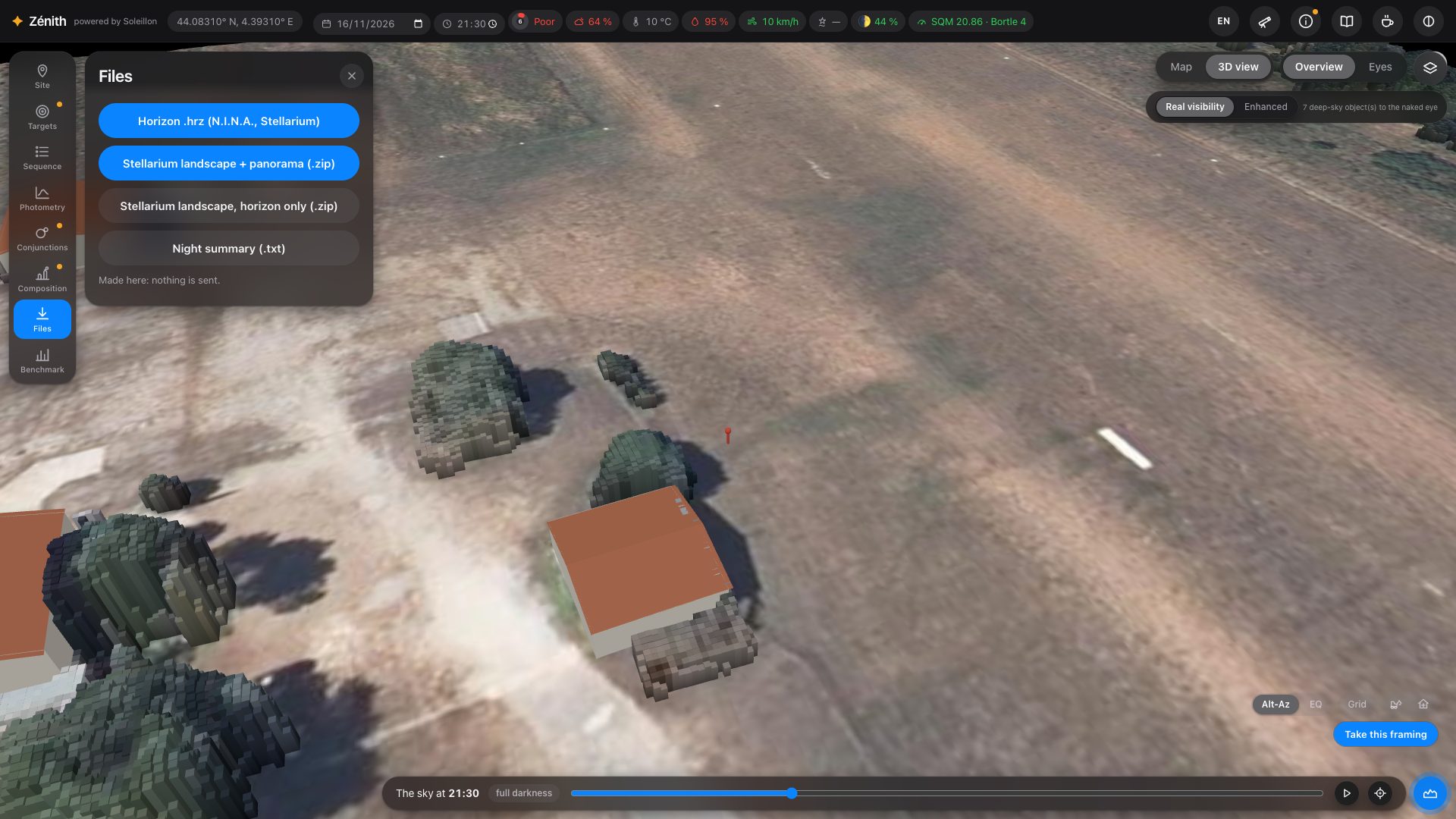
- Horizon .hrz for N.I.N.A. and Stellarium.
- Stellarium landscape, with a 360° panorama of the site, or the horizon line only. In the panorama only the ground and what stands on it are opaque: the sky is transparent, as the format wants, so it shows the planetarium's own sky (in Stellarium, Astro2001…).
- Night summary as plain text.
- The sequence itself is exported from the Sequence panel (section 10).
15. Benchmark: compare before you buy, or before you travel
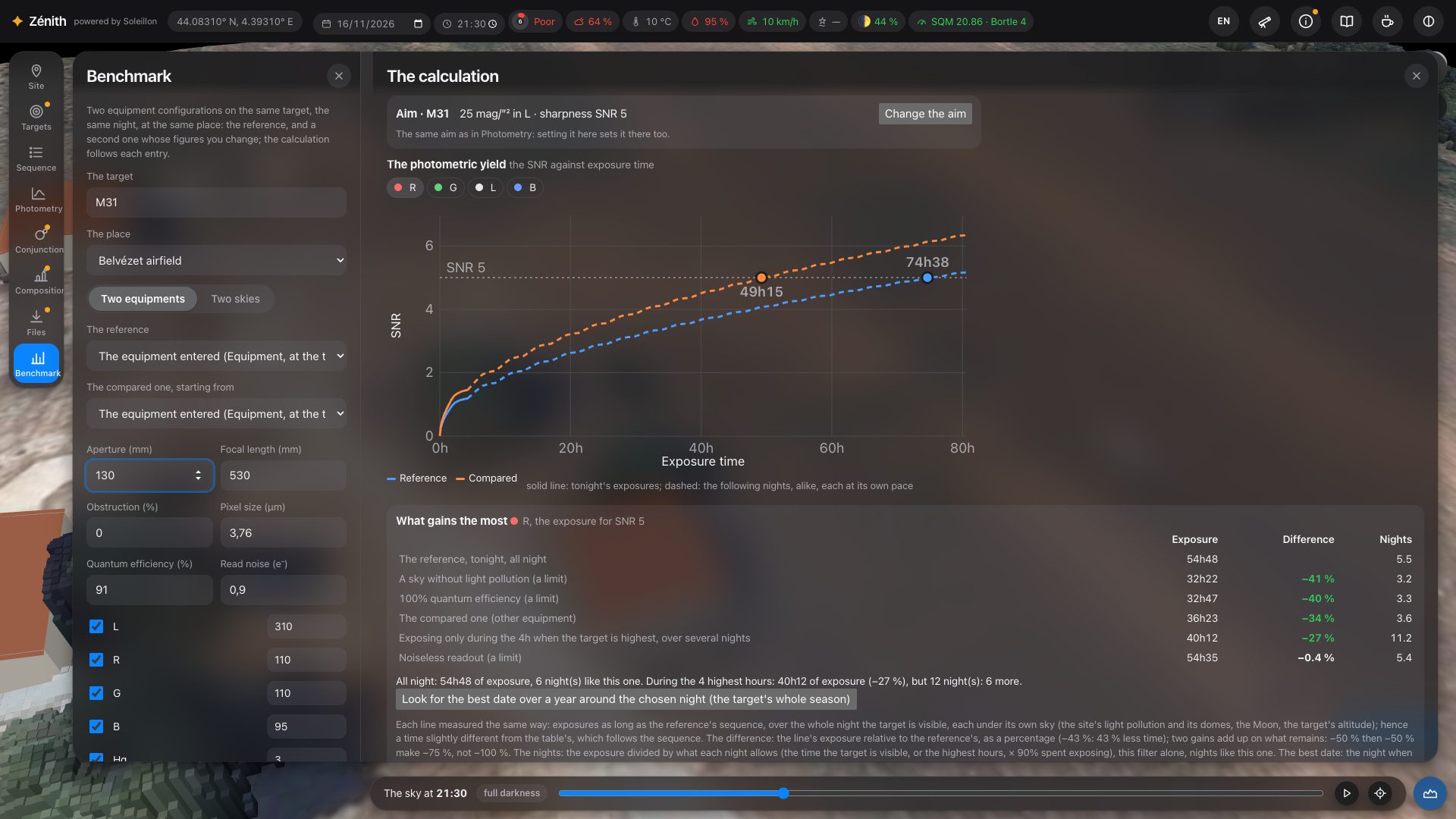
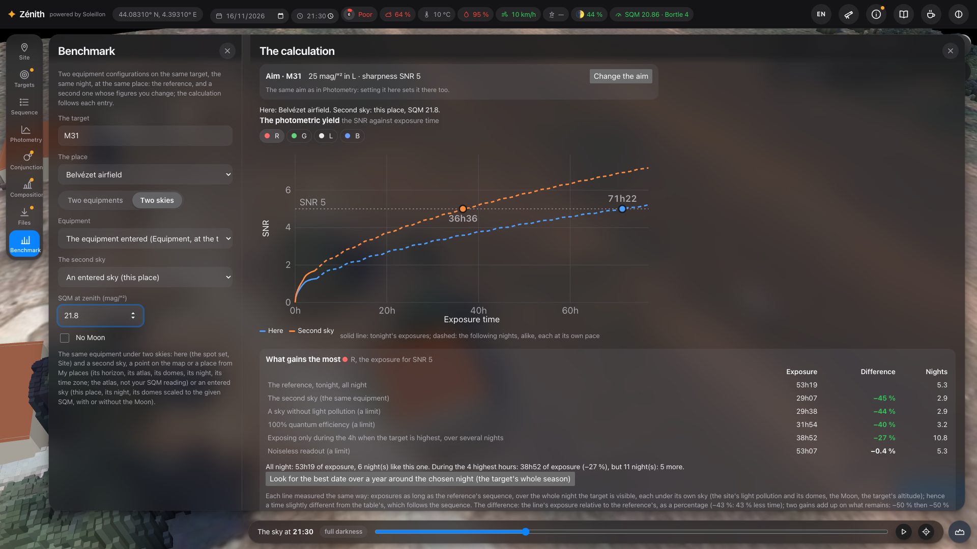
Benchmark, the last button of the left rail (under Files), compares two setups on the same target, at the same place, on the same night, or the same setup under two skies. Each is computed as the Sequence and Photometry panels would: tonight's sequence, its filters and exposures, the sky, the light pollution and domes, the Moon, the forecast aerosols, the real horizon. Never the clouds.
- The target: type its name. The place: your spot (Site) or one of My places.
- Choose Two equipments or Two skies.
- Two equipments: The reference is the equipment entered at the top (Equipment), followed at each change, or a saved setup. The compared one, starting from one of them, gets its own figures in the panel: aperture, focal length, obstruction, pixels, quantum efficiency, read noise, filters and bandwidths. These figures are not kept, and your equipment is not touched.
- Two skies: the reference equipment here, and under The second sky: A point on the map (press Choose the second place on the map, then click: a blue marker; its real horizon, its atlas, its domes, its forecast aerosols, its night and time zone are all computed there), a place from My places (its atlas, never your SQM reading), or An entered sky (this place): your spot with the SQM at zenith you type, and No Moon if you tick it.
The calculation opens in a second panel, The calculation, on the right of the settings, and follows every change. Show the calculation alongside brings it back if you closed it.
What it shows
- The aim (“Aim · M 31: …”), the same as in Photometry. Change the aim unfolds the target's map, the isophote of the extent in yellow ([OIII] along it in cyan), and two sliders: the extent and the target SNR. While you drag, the isophote follows; the benchmark is recomputed when you let go, and Photometry takes up the same aim.
- The photometric yield: the SNR against exposure time, one button per filter, the two setups (or skies) on the same graph. Solid line: tonight's exposures stacked in their order, each under its own sky; dashed: the following nights, alike, each at its own pace (slow when the target is low, fast when it culminates). The line of the target SNR, and the point where each curve reaches it, with its time.
- What gains the most, for the filter of the graph, ranked: the exposure for the target SNR and its difference from the reference tonight, and the nights it takes. The lines: the other setup (or second sky); exposing only during the 4 h when the target is highest, over several nights; the best date of the season, the best one to come and the worst (press Look for the best date over a year around the chosen night (the target's whole season): a year of nights is computed, with the target's season); and three limits: a sky without light pollution, noiseless readout, 100 % quantum efficiency. A sentence weighs up exposing all night against only the high hours: less exposure, but how many more nights.
- The table side by side: light per pixel, F/D, sampling, field; for each filter, the target brightness used, the target and sky signal (e⁻/px/s), tonight's exposure and SNR, the exposure for the target SNR, and the share of each noise (sky, read, target). Then the whole sequence, and what else to change on the compared setup.
Every difference is a percentage of the reference (−43 %: 43 % less time), in green when it improves, in red when it gets worse; under 0.5 %, no colour. Two gains add up on what remains: −50 % then −50 % make −75 %, not −100 %.
16. More tools and tips
- Find the best horizon (Site panel): draw an area of up to 500 m; Zénith tests points inside it and keeps the most open one (avoiding roads and car parks in France).
- Import your horizon (Site panel): a
.hrzfile, thehorizon.txtof a Stellarium landscape, or an “azimuth altitude” CSV. Surveyed with your phone in 30 seconds (for example with Astro Night Companion, free on iPhone), it completes the computed horizon with what the survey may miss. - Correct the terrain (3D view, Overview): cut down trees, add a missing building (section 3).
- Your SQM reading (Information panel) replaces the atlas in every computation.
- Red night mode (last icon of the top bar) keeps your eyes dark-adapted in the field.
- Language: the language button of the top bar, English, Français or Deutsch (section 2); this guide too, in French and German.
- Privacy: no account. Your places, setups, aims and survey tiles stay in your browser. Anonymous statistics are kept to improve Zénith (places rounded to about 1 km, or kept as they are; never published, shared or sold; never an IP address). A SIMBAD report (section 9) records its coordinates, date and town of connection.
17. What is simulated, and the limits
| Part of the sky | Model and data |
|---|---|
| Natural sky | Airglow scaled with the 10.7 cm solar flux of the day (NOAA SWPC; Patat 2008), brighter towards the horizon (van Rhijn); zodiacal light (Leinert et al. 1998); unresolved stars (Gaia DR3); extragalactic light; GAMBONS (Masana et al. 2021). Its spectrum in each filter from ESO's SkyCalc sky model (Noll et al. 2012). |
| Twilight | Patat, Ugolnikov & Postylyakov (2006), from the Sun 5° below the horizon. |
| Light pollution | David Lorenz's atlas (2025) or your SQM reading; light domes from VIIRS, each town at its altitude (Garstang 1986, as given by Cinzano et al. 2000); the lamp spectra of the CIE (CIE 015:2018) through the photopic and scotopic curves and through each filter. |
| Moon | Krisciunas & Schaefer (1991); its colour by distance from the target from ESO's SkyCalc (Jones et al. 2013). Avoidance zone per filter: where its background exceeds 4 times that of the same night without it (otherwise BAIT's Lorentzian rule, as ACP gives it). |
| Extinction | Per filter, at its wavelength: Rayleigh scattering (Bucholtz 1995); aerosols by Ångström's law, forecast by CAMS (Copernicus, via Open-Meteo) or Garstang's clear atmosphere, brought to the altitude of the spot; ozone from SkyCalc; airmass after Krisciunas & Schaefer (1991). |
| The eye | Rod vision weighted by each light's colour, contrast threshold and point-source threshold (Crumey 2014); limiting magnitude per direction. |
| Stars | The Yale Bright Star Catalogue, coloured by their B−V index. |
| Milky Way | Gaia DR3 brightness and colour maps. |
| Display | Ferwerda et al. (1996) on the sRGB reference screen; the stretched sky is an optional, labelled exaggeration. |
| Hα and [OIII] | The Northern Sky Narrowband Survey DR0.2 (Ziegenbalg 2025, CC BY-NC-SA 4.0) north of −16°; the Southern H-Alpha Sky Survey Atlas, SHASSA (Gaustad et al. 2001), for Hα south of it; Finkbeiner's (2003) Hα map as a last resort. |
| Broadband brightness | Pan-STARRS DR1 (STScI) north of −30°, converted to B, V, R after Tonry et al. (2012); the DESI Legacy Imaging Surveys DR10 (Dey et al. 2019, CC BY 4.0) south of it; DSS2 for display. |
| Deep-sky shapes | Outlines and light traced on Pan-STARRS DR1 images; cluster stars from Gaia DR3. |
| Sensors | The SPCC database of Siril (the manufacturers' published response curves); a colour sensor computed colour by colour on its Bayer matrix. |
| Exposure | The CCD equation (target, sky background, read noise, exposures added in quadrature) with the surveys above, your equipment and filters, your real horizon; the minimum exposure of Robin Glover (2017). Clouds enter no computation. |
A model, not a measurement. Clouds are not drawn as a mask, nor counted in any computation. Your screen and room are not the sRGB reference. Every source and assumption is written in the page itself: hover the values, and see the sources under each analysis. Comparisons with what you see and measure in the field are very welcome.